`cleave_by()`: A tidyverse-style `split()`

My issues with `split()` in base R

My prior post on tidyverse split-apply-combined ended with me favouring split + map_dfr as a replacement for group_by + do.
In subsequent posts I looked at the runtime of the split function and the idioscrasies of the split function and saw the following for the Base R split() function:

runtime is quadratic in number of splitting variables
runtime is quadratic in number of groups within each variable
the splitting variable gets recycled if it’s not as long as the data.frame being split
NA levels are dropped from the data

Points [1] and [2] mean that split() really slows down as soon as your data grouping becomes moderately complex.

Point [3] means that it’s easy to shoot yourself in the foot and split the data incorrectly.

Point [4] means that split() will just throw away data that happens to have a level value of NA

Why is there no `split` function in the tidyverse?

According to Hadley on github:

A function that acts rowwise on a data frame doesn’t seem like it should live in purrr.

`cleave_by()` - a tidyverse-style version of`split()`

This is an experiment to create a tidyverse-split split() which avoids the problems listed above. If possible (and with as little work as possible) I want a tidyverse-style split function which

keeps runtimes linear in the number of variables
keeps runtimes linear with respect to the number of groups within each variable.
avoids the recyling of any splitting variable
keeps NA levels

Note: Since I am simply writing a wrapper around the base split() function, I’m never going to be faster than it for simple grouping examples. This is because I’m always doing more work upfront which is not necessary for a small number of grouping variables, and only pays off once the number of groups/levels gets bigger.

#-----------------------------------------------------------------------------
#' tidy version of the base `split()` function
#'
#' @param df data.frame to split
#' @param ... unquoted column names from the 'df' data.frame to specify 
#'            the splitting groups
#'
#' @return list of data.frames, one for each group
#-----------------------------------------------------------------------------
cleave_by <- function(df, ...) {
  stopifnot(inherits(df, "data.frame"))
  
  # use tidyeval to get the names ready for dplyr
  grouping <- quos(...)
  
  # Calculate a single number to represent each group
  group_index <- df %>%
    group_by(!!!grouping) %>%
    group_indices()
  
  # do the split by this single group_index variable and return it
  split(df, group_index)
}

mtcars %>% cleave_by(am, vs)

## $`1`
##                      mpg cyl  disp  hp drat    wt  qsec vs am gear carb
## Hornet Sportabout   18.7   8 360.0 175 3.15 3.440 17.02  0  0    3    2
## Duster 360          14.3   8 360.0 245 3.21 3.570 15.84  0  0    3    4
## Merc 450SE          16.4   8 275.8 180 3.07 4.070 17.40  0  0    3    3
## Merc 450SL          17.3   8 275.8 180 3.07 3.730 17.60  0  0    3    3
## Merc 450SLC         15.2   8 275.8 180 3.07 3.780 18.00  0  0    3    3
## Cadillac Fleetwood  10.4   8 472.0 205 2.93 5.250 17.98  0  0    3    4
## Lincoln Continental 10.4   8 460.0 215 3.00 5.424 17.82  0  0    3    4
## Chrysler Imperial   14.7   8 440.0 230 3.23 5.345 17.42  0  0    3    4
## Dodge Challenger    15.5   8 318.0 150 2.76 3.520 16.87  0  0    3    2
## AMC Javelin         15.2   8 304.0 150 3.15 3.435 17.30  0  0    3    2
## Camaro Z28          13.3   8 350.0 245 3.73 3.840 15.41  0  0    3    4
## Pontiac Firebird    19.2   8 400.0 175 3.08 3.845 17.05  0  0    3    2
## 
## $`2`
##                 mpg cyl  disp  hp drat    wt  qsec vs am gear carb
## Hornet 4 Drive 21.4   6 258.0 110 3.08 3.215 19.44  1  0    3    1
## Valiant        18.1   6 225.0 105 2.76 3.460 20.22  1  0    3    1
## Merc 240D      24.4   4 146.7  62 3.69 3.190 20.00  1  0    4    2
## Merc 230       22.8   4 140.8  95 3.92 3.150 22.90  1  0    4    2
## Merc 280       19.2   6 167.6 123 3.92 3.440 18.30  1  0    4    4
## Merc 280C      17.8   6 167.6 123 3.92 3.440 18.90  1  0    4    4
## Toyota Corona  21.5   4 120.1  97 3.70 2.465 20.01  1  0    3    1
## 
## $`3`
##                 mpg cyl  disp  hp drat    wt  qsec vs am gear carb
## Mazda RX4      21.0   6 160.0 110 3.90 2.620 16.46  0  1    4    4
## Mazda RX4 Wag  21.0   6 160.0 110 3.90 2.875 17.02  0  1    4    4
## Porsche 914-2  26.0   4 120.3  91 4.43 2.140 16.70  0  1    5    2
## Ford Pantera L 15.8   8 351.0 264 4.22 3.170 14.50  0  1    5    4
## Ferrari Dino   19.7   6 145.0 175 3.62 2.770 15.50  0  1    5    6
## Maserati Bora  15.0   8 301.0 335 3.54 3.570 14.60  0  1    5    8
## 
## $`4`
##                 mpg cyl  disp  hp drat    wt  qsec vs am gear carb
## Datsun 710     22.8   4 108.0  93 3.85 2.320 18.61  1  1    4    1
## Fiat 128       32.4   4  78.7  66 4.08 2.200 19.47  1  1    4    1
## Honda Civic    30.4   4  75.7  52 4.93 1.615 18.52  1  1    4    2
## Toyota Corolla 33.9   4  71.1  65 4.22 1.835 19.90  1  1    4    1
## Fiat X1-9      27.3   4  79.0  66 4.08 1.935 18.90  1  1    4    1
## Lotus Europa   30.4   4  95.1 113 3.77 1.513 16.90  1  1    5    2
## Volvo 142E     21.4   4 121.0 109 4.11 2.780 18.60  1  1    4    2

`cleave_by()` keeps NA levels

Creating the groups within cleave_by() uses dplyr::group_by + group_indices.

As both of these functions are aware of (and retain) NA values, using them to create the group labels means that we keep NA levels within a splitting variable.

test_df <- data_frame(a=c(1, 1, 1, 2, 2, 3, NA, NA), b=1:8)

## Warning: `data_frame()` is deprecated, use `tibble()`.
## This warning is displayed once per session.

test_df %>%
  cleave_by(a)

## $`1`
## # A tibble: 3 x 2
##       a     b
##   <dbl> <int>
## 1     1     1
## 2     1     2
## 3     1     3
## 
## $`2`
## # A tibble: 2 x 2
##       a     b
##   <dbl> <int>
## 1     2     4
## 2     2     5
## 
## $`3`
## # A tibble: 1 x 2
##       a     b
##   <dbl> <int>
## 1     3     6
## 
## $`4`
## # A tibble: 2 x 2
##       a     b
##   <dbl> <int>
## 1    NA     7
## 2    NA     8

`cleave_by()` avoids factor recycling

split() allows the user to pass in any splitting variable, and in cases where there is a length mismatch with the number of rows in the original data.frame, it will recycle the values.

With cleave_by(), because we’re using column names of the data.frame to specify the splitting variable, it is always guaranteed to be the same length as the data.frame itself.

Thus, any recycling of the splitting variable is completely avoided.

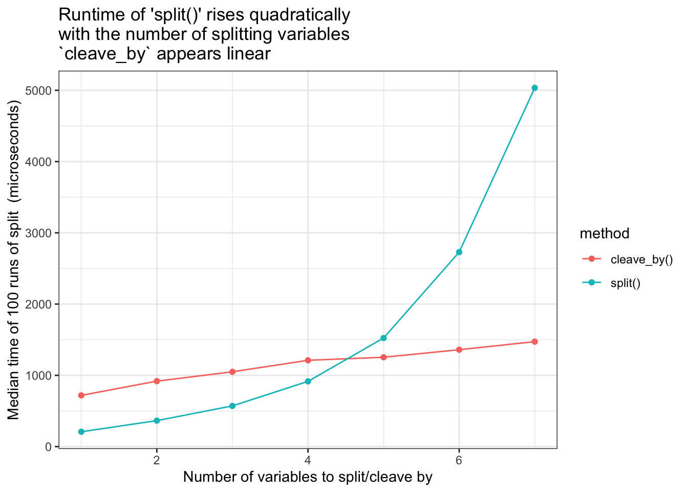
Compare runtimes for increasing number of splitting variables. `cleave_by()` vs `split()`

As seen in the graph below, cleave_by() runtimes appear linear with respect to the number of splitting variables, however it does start at a higher baseline time than split().

test_df <- create_test_df(cols=10, rows=10, levels_per_var=2)  # See appendix for 'create_test_df'

bench <- microbenchmark(
  times = 40,
  split(test_df, test_df[, c('a'                              )]),
  split(test_df, test_df[, c('a', 'b'                         )]),
  split(test_df, test_df[, c('a', 'b', 'c'                    )]),
  split(test_df, test_df[, c('a', 'b', 'c', 'd'               )]),
  split(test_df, test_df[, c('a', 'b', 'c', 'd', 'e'          )]),
  split(test_df, test_df[, c('a', 'b', 'c', 'd', 'e', 'f'     )]),
  split(test_df, test_df[, c('a', 'b', 'c', 'd', 'e', 'f', 'g')]),
  cleave_by(test_df, a),
  cleave_by(test_df, a, b),
  cleave_by(test_df, a, b, c),
  cleave_by(test_df, a, b, c, d),
  cleave_by(test_df, a, b, c, d, e),
  cleave_by(test_df, a, b, c, d, e, f),
  cleave_by(test_df, a, b, c, d, e, f, g)
)

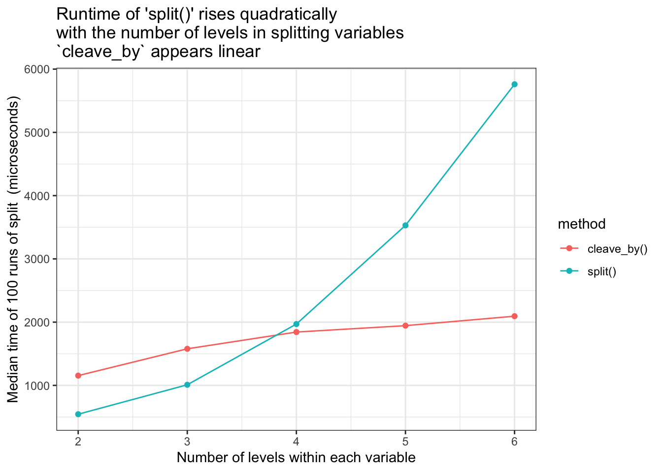
Compare runtimes for increasing number of levels within grouping variables. `cleave_by()` vs `split()`

As seen in the graph below, cleave_by() runtimes appear linear with respect to the number of levels within grouping variables, however it does start at a higher baseline time than split()

test_df2  <- create_test_df(cols=4, rows=40, levels_per_var= 2)  # See appendix for 'create_test_df'
test_df3  <- create_test_df(cols=4, rows=40, levels_per_var= 3)  # See appendix for 'create_test_df'
test_df4  <- create_test_df(cols=4, rows=40, levels_per_var= 4)  # See appendix for 'create_test_df'
test_df5  <- create_test_df(cols=4, rows=40, levels_per_var= 5)  # See appendix for 'create_test_df'
test_df6  <- create_test_df(cols=4, rows=40, levels_per_var= 6)  # See appendix for 'create_test_df'

bench <- microbenchmark(
  split(test_df2 , test_df2[, c('a', 'b', 'c')]),
  split(test_df3 , test_df3[, c('a', 'b', 'c')]),
  split(test_df4 , test_df4[, c('a', 'b', 'c')]),
  split(test_df5 , test_df5[, c('a', 'b', 'c')]),
  split(test_df6 , test_df6[, c('a', 'b', 'c')]),
  cleave_by(test_df2, a, b, c),
  cleave_by(test_df3, a, b, c),
  cleave_by(test_df4, a, b, c),
  cleave_by(test_df5, a, b, c),
  cleave_by(test_df6, a, b, c)
)

Conclusions

Does cleave_by() work?

keeps runtimes linear in the number of variables
- Goal met - the runtime increases linearly not quadratically. But from a higher baseline
- The higher baseline is because of the grouping prep-work which is always done
- This prep-work only pays off when there are more than 4 grouping variables
- Would Rcpp help here?
keeps runtimes linear with respect to the number of groups within each variable.
- Goal met - the runtime increases linearly not quadratically. But from a higher baseline
- The higher baseline is because of the grouping prep-work which is always done
- This prep-work pays off very quickly, and for test dataset cleave_by has the advantage over split() for 4 or more levels per splitting variable.
- Would Rcpp help here?
Avoids the recyling of any splitting variable
- Goal met.
- By only allowing column names to be passed in, if the column name is valid, then the factor length will always be the same as the data.frame length and there will never be value recycling
keeps NA levels
- dplyr::group_by + group_indices are both aware of (and keep) NA values. Using them to create the group labels means that NA levels within a splitting variable are kept.

Future

Would some C++ (via Rcpp) help speed up the baseline case at all?
Some corner cases to test for:
- What should be done with factor columns with empty levels?
- What about data.frames with zero rows or zero cols?
- Can you cleave_by() using a list-column as the splitting variable?

Appendix

set.seed(1)

#-----------------------------------------------------------------------------
#' Create a test data set
#'
#' @param cols how many columns?
#' @param rows how many rows?
#' @param levels_per_col how many distinct levels for each variable/column?
#'
#-----------------------------------------------------------------------------
create_test_df <- function(cols, rows, levels_per_var) {
  data_source <- letters[seq(levels_per_var)]
  
  create_column <- function(...) {sample(data_source, size = rows, replace = TRUE)}
  letters[seq(cols)] %>% 
    set_names(letters[seq(cols)]) %>%
    purrr::map_dfc(create_column) 
}

`cleave_by()`: A tidyverse-style `split()`

My issues with split() in base R

Why is there no split function in the tidyverse?

cleave_by() - a tidyverse-style version ofsplit()

cleave_by() keeps NA levels

cleave_by() avoids factor recycling

Compare runtimes for increasing number of splitting variables. cleave_by() vs split()

Compare runtimes for increasing number of levels within grouping variables. cleave_by() vs split()