Hilbert curves with an ad-hoc L-system
Today in my ongoing quest to generate fractals in Rstats using every available avenue: generating a hilbert curve using an ad-hoc L-system
Methods for generating fractals so far:
- Sierpinski Triangle in plotmath
- Another sierpinski triangle in plotmath
- Sierpinski triangle using character strings
- Using R matrices to create a sierpinski carpet
- Today: Generating hilbert curves with an ad-hoc L-system
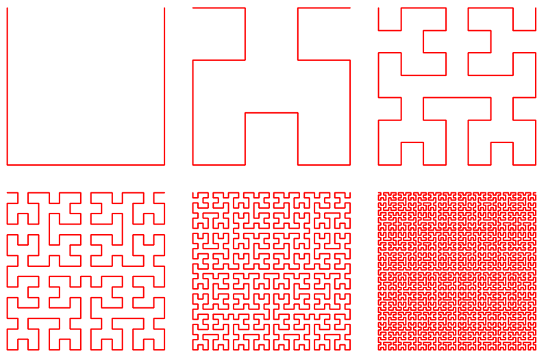
Hilbert Curve
A Hilbert Curve is a fractal space-filling curve that looks like a classic 70s wallpaper pattern.
L-systems
L-systems consist of:
- Alphabet - the set of symbols to be manipulated
- Axiom - the initial state of the system
- Production Rules - how to map from one state to the next
- Rendering
That is, starting with an axiom, subsequent iterations are generated by applying the Production Rules over and over. Once the required number of iterations are performed, the vector of alphabet characters is rendered graphically (somehow!)
Hilbert curves using L-system
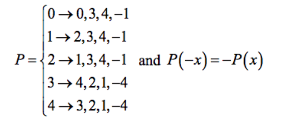
I’m following the L-system for Hilbert curves as described in Arie Bos’ paper.
The alphabet -
- 0 - start code
- 1/-1 - right/left
- 2/-2 - up/down
- 3/-3 - right/left
- 4/-4 - up/down
Production rules:
#~~~~~~~~~~~~~~~~~~~~~~~~~~~~~~~~~~~~~~~~~~~~~~~~~~~~~~~~~~~~~~~~~~~~~~~~~~~~~
# 2. Axiom
#~~~~~~~~~~~~~~~~~~~~~~~~~~~~~~~~~~~~~~~~~~~~~~~~~~~~~~~~~~~~~~~~~~~~~~~~~~~~~
axiom  <- c(0)

#~~~~~~~~~~~~~~~~~~~~~~~~~~~~~~~~~~~~~~~~~~~~~~~~~~~~~~~~~~~~~~~~~~~~~~~~~~~~~
# 3. Production rules
#~~~~~~~~~~~~~~~~~~~~~~~~~~~~~~~~~~~~~~~~~~~~~~~~~~~~~~~~~~~~~~~~~~~~~~~~~~~~~
pr <- list(
  '-4' = -c(3, 2, 1, -4),
  '-3' = -c(4, 2, 1, -4),
  '-2' = -c(1, 3, 4, -1),
  '-1' = -c(2, 3, 4, -1),
   '0' =  c(0, 3, 4, -1),
   '1' =  c(2, 3, 4, -1),
   '2' =  c(1, 3, 4, -1),
   '3' =  c(4, 2, 1, -4),
   '4' =  c(3, 2, 1, -4)
)

#~~~~~~~~~~~~~~~~~~~~~~~~~~~~~~~~~~~~~~~~~~~~~~~~~~~~~~~~~~~~~~~~~~~~~~~~~~~~~
# Function to apply the Production rule
# i.e. lookup each current character and replace it with the
#      nominated 4 characters
#~~~~~~~~~~~~~~~~~~~~~~~~~~~~~~~~~~~~~~~~~~~~~~~~~~~~~~~~~~~~~~~~~~~~~~~~~~~~~
T <- . %>% purrr::map(~pr[[as.character(.x)]]) %>% flatten_dbl()

#~~~~~~~~~~~~~~~~~~~~~~~~~~~~~~~~~~~~~~~~~~~~~~~~~~~~~~~~~~~~~~~~~~~~~~~~~~~~~
# Apply the production rule a number of times
#~~~~~~~~~~~~~~~~~~~~~~~~~~~~~~~~~~~~~~~~~~~~~~~~~~~~~~~~~~~~~~~~~~~~~~~~~~~~~
H <- T(T(T(T(T(T(axiom))))))

#~~~~~~~~~~~~~~~~~~~~~~~~~~~~~~~~~~~~~~~~~~~~~~~~~~~~~~~~~~~~~~~~~~~~~~~~~~~~~
# Table to interpret the alphabet in terms of x,y offsets
#~~~~~~~~~~~~~~~~~~~~~~~~~~~~~~~~~~~~~~~~~~~~~~~~~~~~~~~~~~~~~~~~~~~~~~~~~~~~~
dh <- tribble(
  ~H, ~x, ~y,
  -4,  0, -1,
  -3, -1,  0,
  -2,  0, -1,
  -1, -1,  0,
   0,  0,  0,
   1,  1,  0,
   2,  0,  1,
   3,  1,  0,
   4,  0,  1
)

#~~~~~~~~~~~~~~~~~~~~~~~~~~~~~~~~~~~~~~~~~~~~~~~~~~~~~~~~~~~~~~~~~~~~~~~~~~~~~
# Map the entire string to a path of points
#~~~~~~~~~~~~~~~~~~~~~~~~~~~~~~~~~~~~~~~~~~~~~~~~~~~~~~~~~~~~~~~~~~~~~~~~~~~~~
dha <- dh %>%
  right_join(data_frame(H=H), by='H') %>%
  mutate(
    x = cumsum(x),
    y = cumsum(y)
  )
Warning: `data_frame()` is deprecated, use `tibble()`.
This warning is displayed once per session.#~~~~~~~~~~~~~~~~~~~~~~~~~~~~~~~~~~~~~~~~~~~~~~~~~~~~~~~~~~~~~~~~~~~~~~~~~~~~~
# Plot it!
#~~~~~~~~~~~~~~~~~~~~~~~~~~~~~~~~~~~~~~~~~~~~~~~~~~~~~~~~~~~~~~~~~~~~~~~~~~~~~
ggplot(dha) +
geom_path(aes(x, y)) +
theme_void() +
coord_fixed()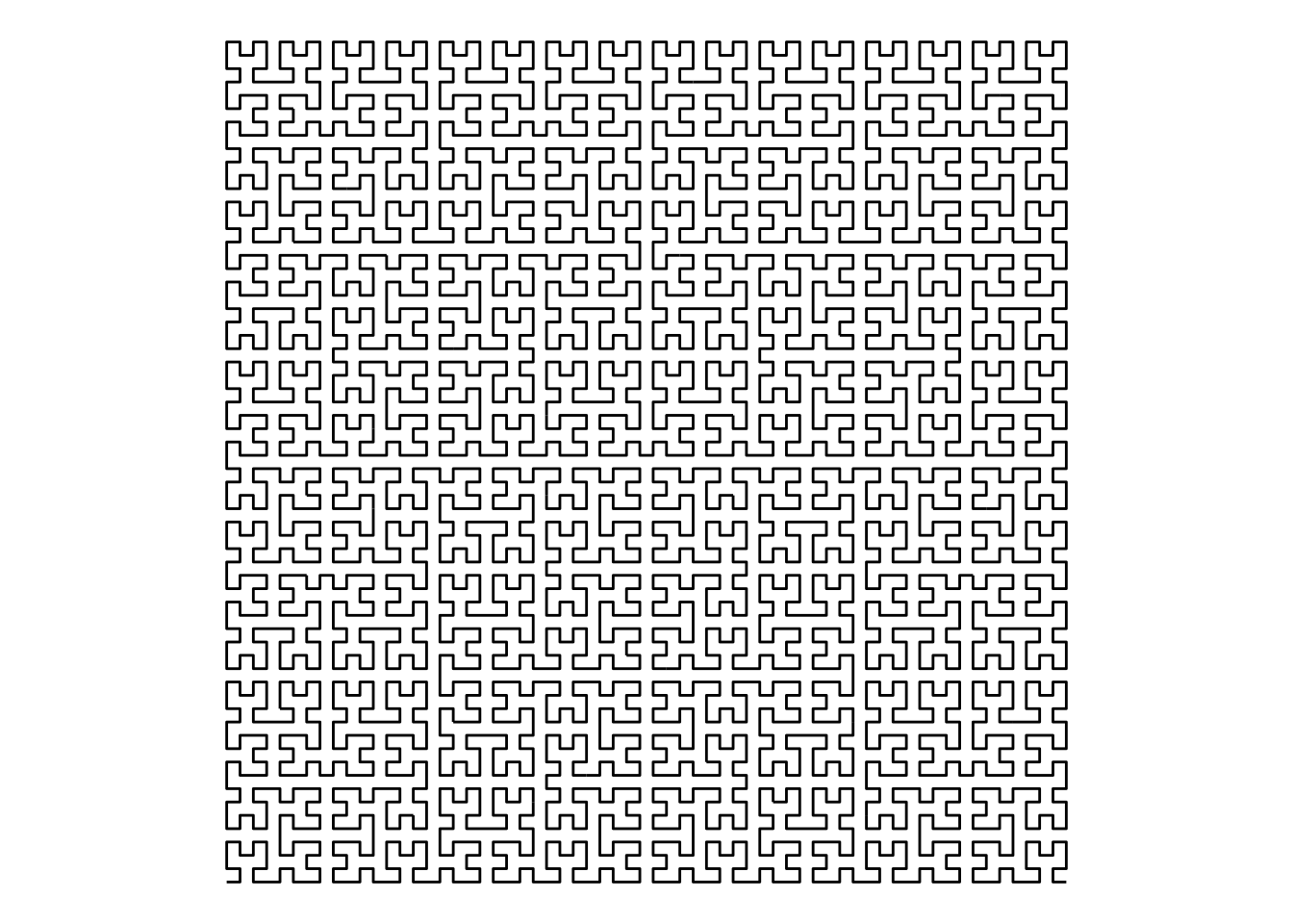
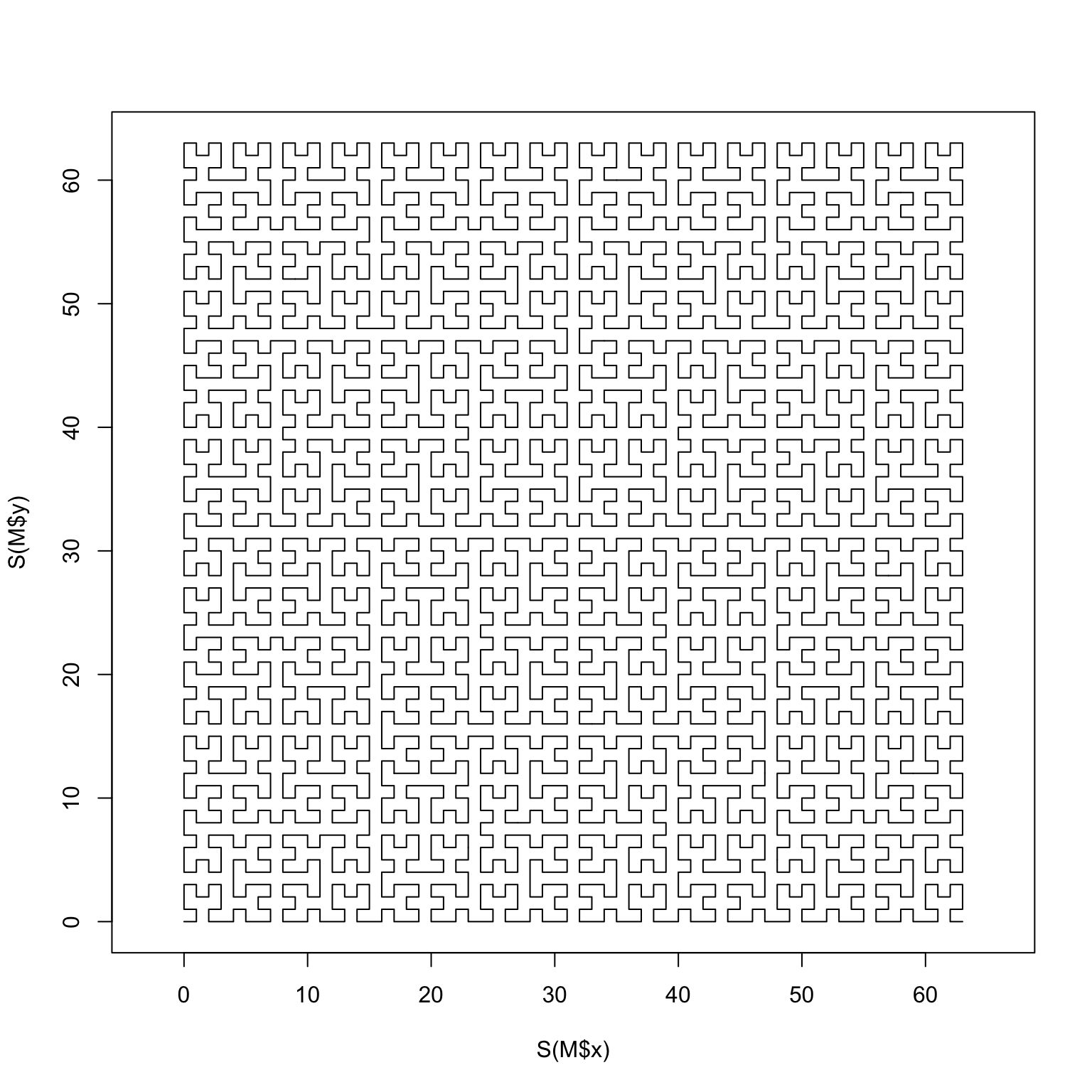
Tweetable Version - Hilbert curves in 2D using L-system
#rstats
library(tidyverse)
A=B=c(2,3,4,-1)
B[1]=1
C=D=c(4,2,1,-4)
D[1]=3
T=.%>%map(~list(-D,-C,-B,-A,c(0,3,4,-1),A,B,C,D)[.x+5])%>%unlist
E=c(0,1,0,1);G=rev(E);M=tibble(H=-4:4,x=c(-E,0,G),y=c(-G,0,E))
M=M[match(T(T(T(T(T(T(0)))))),M$H),-1]
S=cumsum
plot(S(M$x),S(M$y),t='l',as=1)