gganimate with bitmap fonts

Bitmap fonts

In a bitmap font, a character is defined by a binary matrix - where the matrix is 1 the underlying pixel is turned on, otherwise it is turned off.

An example matrix of an 8x8 binary matrix to define the letter a is shown below:

     [,1] [,2] [,3] [,4] [,5] [,6] [,7] [,8]
[1,]    0    0    0    0    0    0    0    0
[2,]    0    0    0    0    0    0    0    0
[3,]    0    0    1    1    1    1    0    0
[4,]    0    0    0    0    0    1    1    0
[5,]    0    0    1    1    1    1    1    0
[6,]    0    1    1    0    0    1    1    0
[7,]    0    0    1    1    1    1    1    0
[8,]    0    0    0    0    0    0    0    0

This matrix can be easily plotted with the raster package

withr::with_package('raster', {
  plot(raster(char_matrix$a), col=c(1,0), legend=FALSE, ann=FALSE, axes=FALSE)
})

Rather than individually creating bitmap font matrices, I’m actually reading in bitmap font files from disk. I haven’t packaged that code up yet, but hopefully will do so soon. For this post I’ll just use some manually created character data stored in char_df.

Rendering a bitmap font character with ggplot2

To work with ggplot2, the matrix for an 8x8 character is turned into a data.frame.

The data.frame is the x and y co-ordinates of all the locations of 1 in the bitmap matrix.

Here is a data.frame for the same a, now ready for ggplot2.

   x y
1  2 5
2  3 5
3  4 5
4  5 5
5  5 4
6  6 4
7  2 3
8  3 3
9  4 3
10 5 3
11 6 3
12 1 2
13 2 2
14 5 2
15 6 2
16 2 1
17 3 1
18 4 1
19 5 1
20 6 1

This data.frame is plotted using ggplot2::geom_tile()

ggplot(char_df$a, aes(x, y)) + 
  geom_tile() + 
  coord_equal() +
  theme_minimal()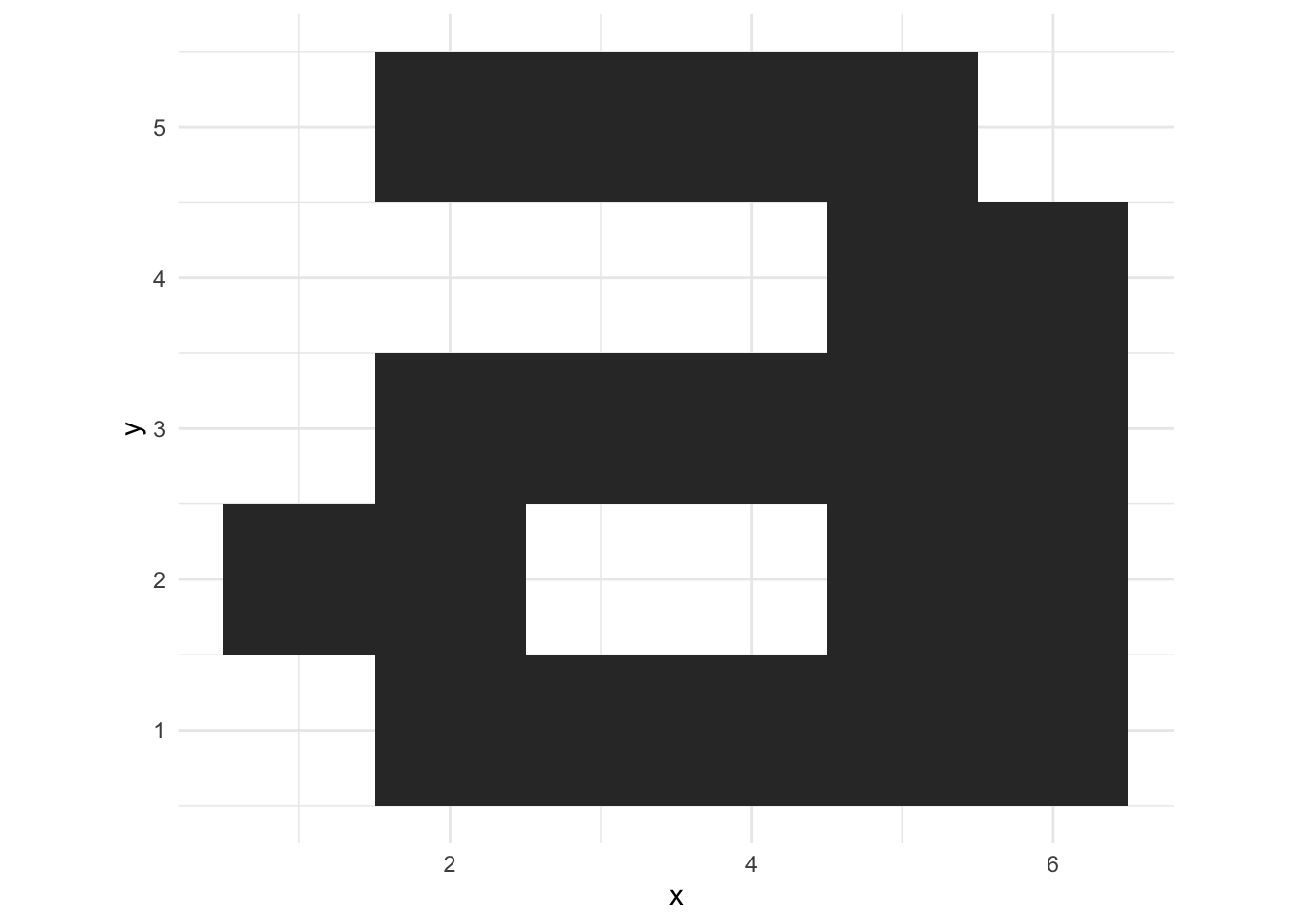

The tile size is set a bit smaller than 1 to get the retro pixel look:

ggplot(char_df$a, aes(x, y)) + 
  geom_tile(width=0.9, height=0.9) + 
  coord_equal() +
  theme_minimal()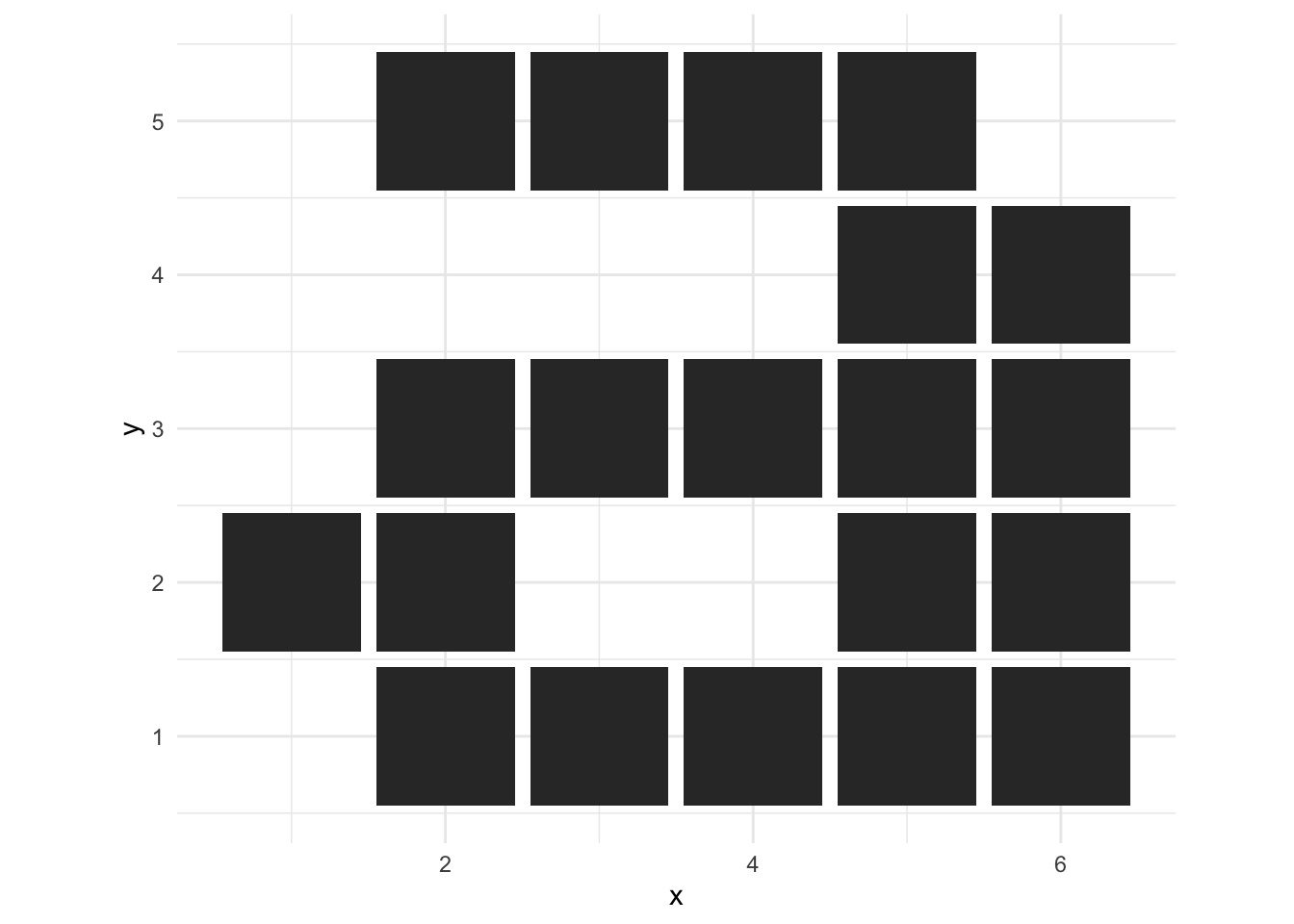

Preparing a data.frame for gganimate

The data.frame for gganimate is going to consist of 3 characters (a, b, c), displayed one-at-a-time.

• Create a data.frame for each bitmap character
• Give each character an idx which will let gganimate control when it is displayed
• Stack them all into a single data.frame with dplyr::bind_rows()

plot_df <- dplyr::bind_rows(
  char_df$a %>% mutate(idx = 1),
  char_df$b %>% mutate(idx = 2),
  char_df$c %>% mutate(idx = 3)
)

Plotting without gganimate results in the 3 letters being superimposed. Not really very useful, but a stepping stone to the actual animation.

p <- ggplot(plot_df, aes(x, y)) + 
  geom_tile(width=0.9, height=0.9) + 
  coord_equal() +
  theme_minimal()

p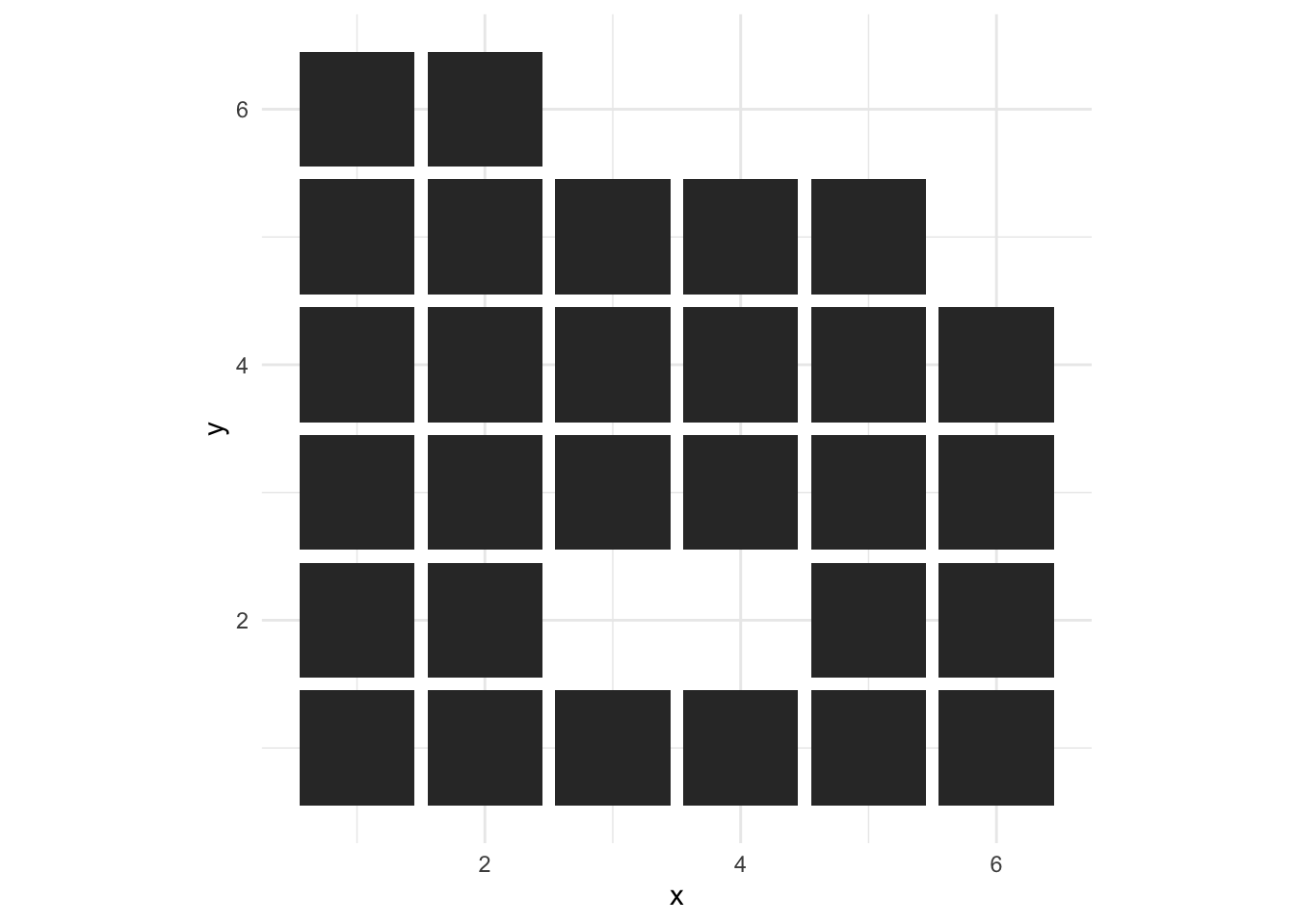

Below I facet by idx to separate out each character in space. gganimate will use the idx column to separate the characters in time using transition_states().

p + 
  facet_wrap(~idx) + 
  theme_bw()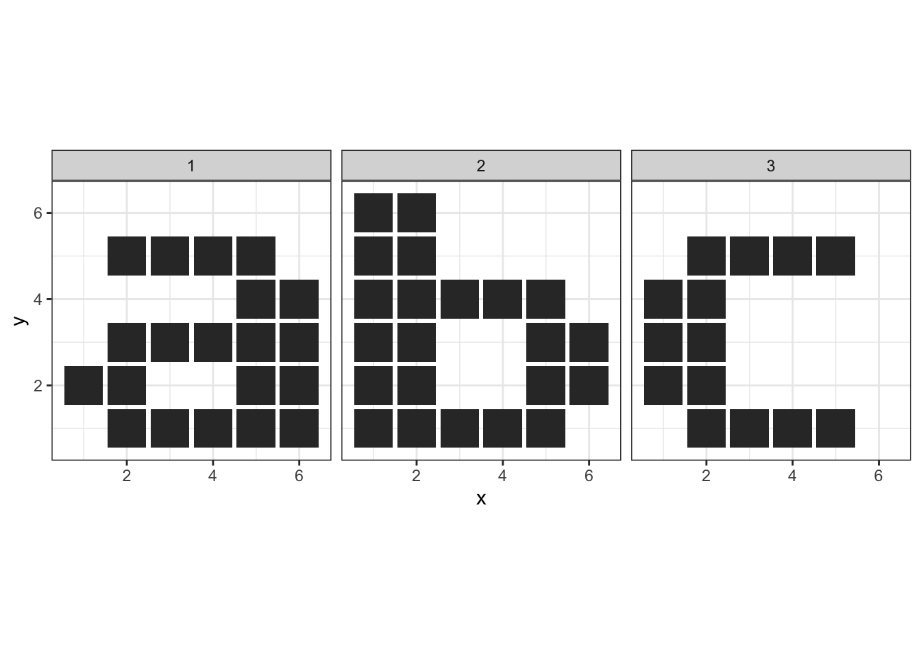 

Plotting with gganimate - facetting in time!

gganimate takes a standard ggplot and separates out the individual states (i.e. the idx variable) by rendering them at different times.

By analogy:

• ggplot2::facet_wrap() renders the data at different locations in space dependent upon the facetting variable
• gganimate::transition_states() renders the data at different times dependent upon the states variable.

panim <- p +
  transition_states(
    states            = idx, # variable in data
    transition_length = 1,   # all states display for 1 time unit
    state_length      = 1    # all transitions take 1 time unit
  ) +
  enter_fade() +             # How new blocks appear
  exit_fade() +              # How blocks disappear
  ease_aes('sine-in-out')    # Tweening movement

panim

Controlling the animation length and image size

By default, the animation is scaled into 100 frames of PNG output at 10 frames-per-second. These png files are then rendered to an animated gif using gifski.

By default the individual images are rendered using R’s built-in png() which has a default output size of 480x480 pixels.

To render the gif differently (e.g. shorter duration, faster playback, smaller image size), you can call animate() directly on the plot object

animate(panim, fps=20, nframes=50, width=200, height=200)

To Do

• Package up the code for parsing bitmap font files