threed - drawing a cube in ggplot2

Introduction

This post explores how to plot a cube in ggplot2 using the threed library.

ggplot2 doesn’t include any notion of a 3rd spatial axis, so instead, after manipulating a 3d object, we use perspective projection to “flatten” its faces and vertices onto a 2d plane. These projected faces/vertices are what ggplot2 will plot.

Prepare an object for plotting

• Create an object (here the standard 2x2x2 cube is being used)
• Define where camera is located, and where it is looking
• Transform the object into camera space
• Perspective transform the data

#~~~~~~~~~~~~~~~~~~~~~~~~~~~~~~~~~~~~~~~~~~~~~~~~~~~~~~~~~~~~~~~~~~~~~~~~~~~~~~
# The `threed` package has some builtin objects in `threed::mesh3dobj`
#~~~~~~~~~~~~~~~~~~~~~~~~~~~~~~~~~~~~~~~~~~~~~~~~~~~~~~~~~~~~~~~~~~~~~~~~~~~~~~
obj <- threed::mesh3dobj$cube

#~~~~~~~~~~~~~~~~~~~~~~~~~~~~~~~~~~~~~~~~~~~~~~~~~~~~~~~~~~~~~~~~~~~~~~~~~~~~~~
# Define camera 'lookat' matrix i.e. camera-to-world transform
#~~~~~~~~~~~~~~~~~~~~~~~~~~~~~~~~~~~~~~~~~~~~~~~~~~~~~~~~~~~~~~~~~~~~~~~~~~~~~~
camera_to_world <- threed::look_at_matrix(eye = c(1.5, 1.75, 4), at = c(0, 0, 0))

#~~~~~~~~~~~~~~~~~~~~~~~~~~~~~~~~~~~~~~~~~~~~~~~~~~~~~~~~~~~~~~~~~~~~~~~~~~~~~~
# Transform the object into camera space and do perspective projection
#~~~~~~~~~~~~~~~~~~~~~~~~~~~~~~~~~~~~~~~~~~~~~~~~~~~~~~~~~~~~~~~~~~~~~~~~~~~~~~
obj <- obj %>%
  transform_by(invert_matrix(camera_to_world)) %>%
  perspective_projection()

as.data.frame(obj) %>% knitr::kable()

Plot the points for the vertices of the object

• threed defines a fortify.mesh3d() function.
• If a mesh3d object is given as the data for aggplot2 call, ggplot2 will automatically use fortify() to convert into a data.frame.
• i.e. because threed defines fortify.mesh3d(), we can call ggplot2 directly with a mesh3d object.

ggplot(obj, aes(x, y)) +
  geom_point() +
  theme_void() +
  theme(legend.position = 'none') +
  coord_equal()

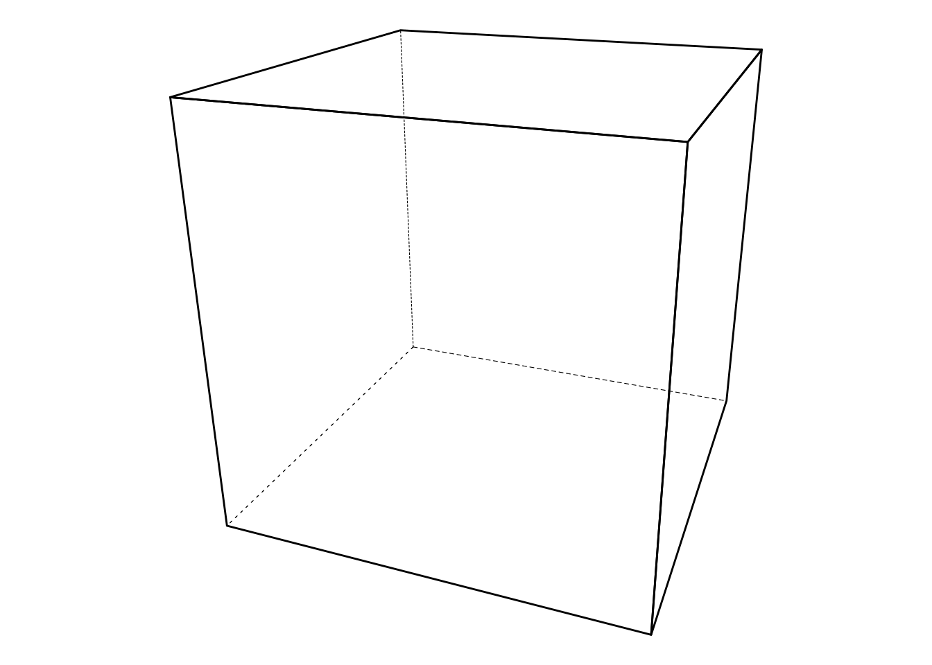
Plot the outline of each polygon

• Each element has a unique element_id, and this is used as the group aesthetic to inform ggplot that it should draw one polygon for each element.
• Set fill = NA, colour = 'black' to draw only the borders of each polygon.

ggplot(obj, aes(x, y, group = element_id)) +
  geom_polygon(fill = NA, colour = 'black', size = 0.2) +
  theme_void() +
  theme(legend.position = 'none') +
  coord_equal()

Dotted rendering of hidden lines

• To draw hidden elements in a different way, use the hidden variable.
• hidden is a boolean variable indicating if a triangle or quad element is facing away from the camera.
• Here a different linetype is used for hidden elements

ggplot(obj, aes(x, y, group = element_id)) +
  geom_polygon(fill = NA, colour='black', aes(linetype = hidden,  size = hidden)) +
  scale_linetype_manual(values = c('TRUE' = "dotted", 'FALSE' = 'solid')) +
  scale_size_manual(values = c('TRUE' = 0.2, 'FALSE' = 0.5)) +
  theme_void() +
  theme(legend.position = 'none') +
  coord_equal()

Hidden line removal

• Here a zero-width linetype is used for hidden elements to hide them.

ggplot(obj, aes(x, y, group = element_id)) +
  geom_polygon(fill = NA, colour = 'black', aes(size = hidden)) +
  scale_size_manual(values = c('TRUE' = 0, 'FALSE' = 0.5)) +
  theme_void() +
  theme(legend.position = 'none') +
  coord_equal()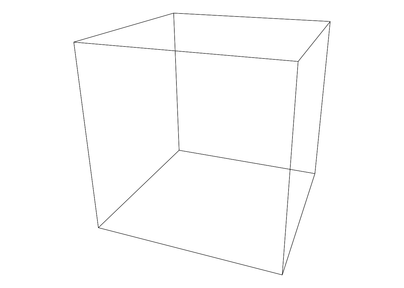

Naive Filled Polygons

• When filling polygons, ggplot2 will draw them in the order of the group variable.
• If we group by element_id then the polygons are drawn in the order in which they were defined. This means that polygons which are further away will be draw over the top of ones which are actually close to the eye.
  
• The result will look weird - Almost Escher-esque!

ggplot(obj, aes(x, y, group = element_id)) +
  geom_polygon(fill = 'lightblue', colour = 'black', size = 0.2) +
  theme_void() +
  theme(legend.position = 'none') +
  coord_equal()

Filled Polygons - (1) Drop hidden elements so they never get drawn

• First method for drawing filled polygons:
  • drop hidden elements manually
  • Do this by explicitly converting the mesh3d object to a data.frame, and then filtering to keep only the elements which aren’t hidden.
• For mesh3d objects converted to data.frames, hidden is defined as TRUE for any face which has a normal which points towards the negative Z axis (i.e. away from the viewing plane).

obj_df <- as.data.frame(obj) %>%
  filter(!hidden)

ggplot(obj_df, aes(x, y, group = element_id)) +
  geom_polygon(fill = 'lightblue', colour = 'black', size = 0.2) +
  theme_void() +
  theme(legend.position = 'none') +
  coord_equal()

Filled Polygons - (2) Assign hidden elements a fill of NA so they get drawn invisibly

• Second method for drawing filled polygons:
  • draw hidden elements invisibly
  • Do this by explicitly converting the mesh3d object to a data.frame, and then manually setting the variables mapped to fill and colour to be NA for hidden elements

obj_df <- as.data.frame(obj) %>%
  mutate(
    shade      = ifelse(hidden, NA, 'lightblue'),
    linecolour = ifelse(hidden, NA, 'black')
  )

ggplot(obj_df, aes(x, y, group = element_id)) +
  geom_polygon(aes(fill = I(shade), colour = I(linecolour)), size = 0.2) +
  theme_void() +
  theme(legend.position = 'none') +
  coord_equal()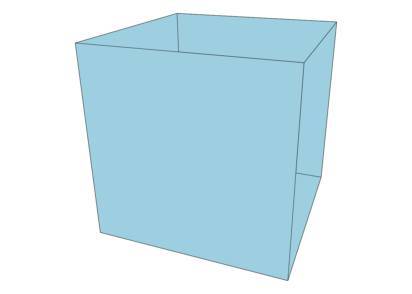 

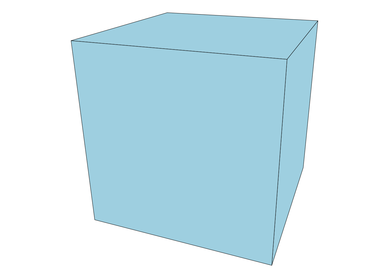
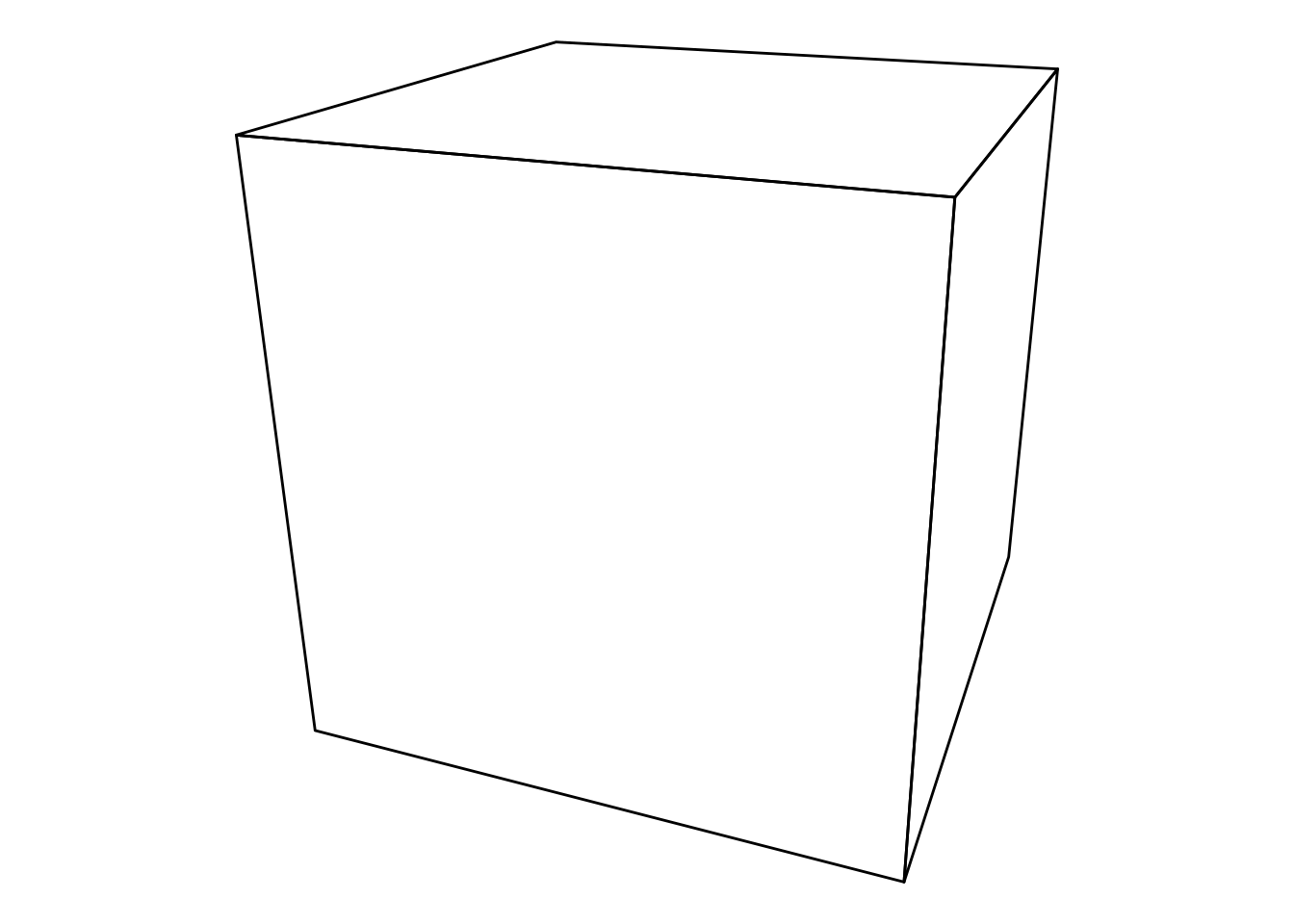
Filled Polygons - (3) Use the zorder variable to control draw order

• Third method for drawing filled polygons:
  • Draw the elements from furtherest to nearest
  • Exploit the fact that elements are drawn in the order of the group variable.
  • When converting a mesh3d to a data.frame, a zorder variable is created starting at 1 for the furtherest element, up to n for the closest element.
  • i.e. change the group variable from element_id to zorder

ggplot(obj, aes(x, y, group = zorder)) +
  geom_polygon(fill = 'lightblue', colour='black', size = 0.2) +
  theme_void() +
  theme(legend.position = 'none') +
  coord_equal()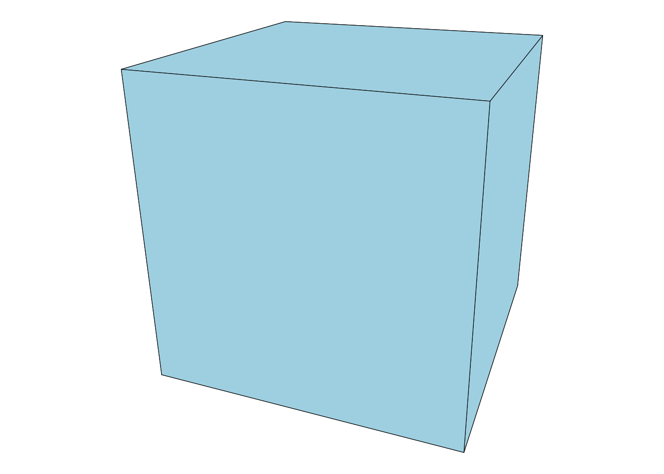 

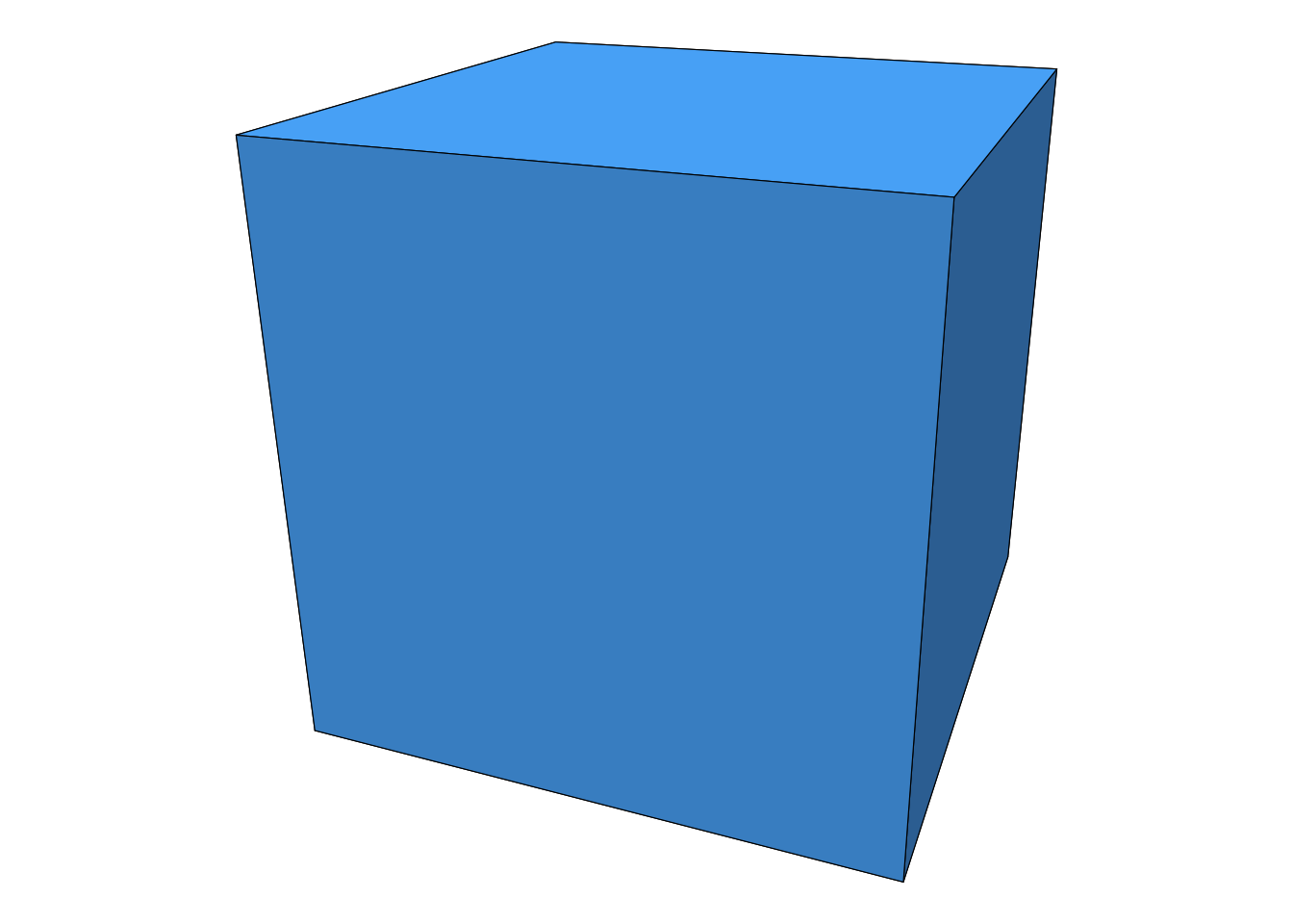
Fake-shaded polygon

• The normal to each face is included in the data.frame representation as fnx, fny, fnz
• By calculating dot products to a light source positioned in the scene, the fraction illumination could be calculated for each element.
• Here, the shading is being completely faked by using the sum fny + fnz to shade the polygons.

ggplot(obj, aes(x, y, group = zorder)) +
  geom_polygon(aes(fill = fny + fnz), colour = 'black', size = 0.2) +
  theme_void() +
  theme(legend.position = 'none') +
  coord_equal()