Puzzle solving - Dominosa
Dominosa is a game/puzzle from Simon Tathams’ Portable Puzzle Collection.
In Dominosa there is a complete set of dominoes up to a certain number (A
classic domino set goes from 0, 0 up to 6, 6). The initial board represents
the dominoes laid out in a grid - we have the numbers, but not the outline of the dominos.
The aim of the puzzle is to determine the locations/orientations of all the dominos so that every possible domino appears exactly once.
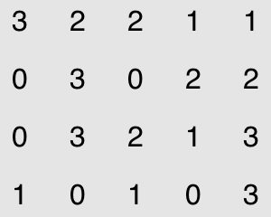
In the images below, the left-hand image is the beginning puzzle board,
the right-hand image is the solution. (Note: For this example, I’m using a smaller board which
only includes all dominos from 0, 0 up to 3, 3)
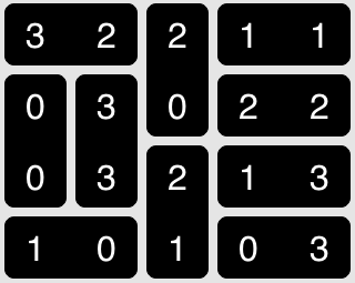
As can be seen in the solution there are 10 distinct tiles in the solution.
These span from 0, 0 up to 3, 3 with each tile only appearing once.
Representation of puzzle and solution in R
The puzzle grid will be represented by a matrix the same dimensions as the grid.
grid <- matrix(as.integer(c(
  3, 2, 2, 1, 1,
  0, 3, 0, 2, 2,
  0, 3, 2, 1, 3,
  1, 0, 1, 0, 3
)), byrow = TRUE, nrow = 4)

grid
[,1] [,2] [,3] [,4] [,5]
[1,] 3 2 2 1 1
[2,] 0 3 0 2 2
[3,] 0 3 2 1 3
[4,] 1 0 1 0 3create_dominosa_plot(grid)
The solution will be represented as a matrix with the following structure:
- An integer matrix of size N x 3. Where N = number of dominoes in puzzle.
- Each row represents one domino
- The
rownameof a row is the pair of numbers on this domino (in sorted order) - The
rowandcolare the starting location for the domino (i.e. the upper-left-most position of the domino) directionindicates whether the domino is horizontal (direction = 0) or vertical (direction = 1)
The solution to the example problem is shown below.
sol row col direction
00 2 1 1
01 4 1 0
02 1 3 1
03 4 4 0
11 1 4 0
12 3 3 1
13 3 4 0
22 2 4 0
23 1 1 0
33 2 2 1create_dominosa_plot(grid, sol)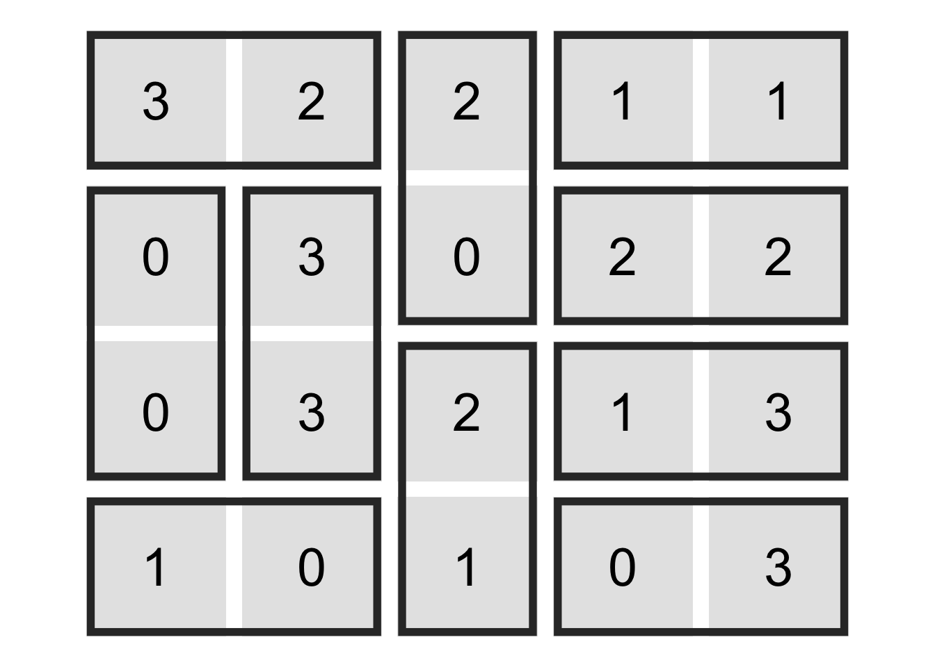
Solver
The solver is implemented via recursion with backtracking. NA is used to mark
grid locations which are already part of a potential solution, and are also used to
mark out-of-bounds areas (off the edge of the initial grid).
At every location try and place a tile both horizontally and vertically. If both
of the grid locations are not NA then place a tile, add it to the solution and
recurse to the next level.
#~~~~~~~~~~~~~~~~~~~~~~~~~~~~~~~~~~~~~~~~~~~~~~~~~~~~~~~~~~~~~~~~~~~~~~~~~~~~~
#' Recursive solver with backtracking
#'
#' @param grid grid of numbers. NA indicates out-of-bounds or that location is already
#'             part of the solution.
#' @param row current row
#' @param col current col
#' @param sol current solutuion. Nx3 matrix.
#~~~~~~~~~~~~~~~~~~~~~~~~~~~~~~~~~~~~~~~~~~~~~~~~~~~~~~~~~~~~~~~~~~~~~~~~~~~~~
solve_dominosa_core <- function(grid, row = 1L, col = 1L, sol = NULL) {

  #~~~~~~~~~~~~~~~~~~~~~~~~~~~~~~~~~~~~~~~~~~~~~~~~~~~~~~~~~~~~~~~~~~~~~~~~~~~
  # If the entire matrix 'grid' is NA, then all positions are consumed into
  # dominoes, and we have a solution!  Return in sorted order.
  #~~~~~~~~~~~~~~~~~~~~~~~~~~~~~~~~~~~~~~~~~~~~~~~~~~~~~~~~~~~~~~~~~~~~~~~~~~~
  if (all(is.na(grid))) {
    sol <- sol[order(rownames(sol)),]
    return(sol)
  }

  #~~~~~~~~~~~~~~~~~~~~~~~~~~~~~~~~~~~~~~~~~~~~~~~~~~~~~~~~~~~~~~~~~~~~~~~~~~~
  # If we're off the end of a row, then jump to the start of the next row
  # If we're off the bottom of 'grid', then we're out of bounds without a solution
  #~~~~~~~~~~~~~~~~~~~~~~~~~~~~~~~~~~~~~~~~~~~~~~~~~~~~~~~~~~~~~~~~~~~~~~~~~~~
  if (col > ncol(grid) - 1L) {col <- 1L;  row <- row + 1L}
  if (row > nrow(grid) - 1L) {stop("Out of bounds. No solution found")}

  #~~~~~~~~~~~~~~~~~~~~~~~~~~~~~~~~~~~~~~~~~~~~~~~~~~~~~~~~~~~~~~~~~~~~~~~~~~~
  # If the current position is NA, then it has already been consumed into a
  # domino, so just jump over to the next one
  #~~~~~~~~~~~~~~~~~~~~~~~~~~~~~~~~~~~~~~~~~~~~~~~~~~~~~~~~~~~~~~~~~~~~~~~~~~~
  if (is.na(grid[row, col])) {
    res <- solve_dominosa_core(grid, row, col + 1L, sol)
    return(res)
  }

  #~~~~~~~~~~~~~~~~~~~~~~~~~~~~~~~~~~~~~~~~~~~~~~~~~~~~~~~~~~~~~~~~~~~~~~~~~~~
  # Next tile oriented horizontally
  #~~~~~~~~~~~~~~~~~~~~~~~~~~~~~~~~~~~~~~~~~~~~~~~~~~~~~~~~~~~~~~~~~~~~~~~~~~~
  pair      <- grid[row, col + 0:1]
  pair_name <- paste(sort(pair), collapse = '')
  if (all(!is.na(pair)) && !pair_name %in% rownames(sol)) {
    # Add the current location+direction to the solution matrix
    this_sol <- matrix(c(row, col, 0L), nrow = 1L)
    rownames(this_sol) <- pair_name
    next_sol <- rbind(sol, this_sol)

    # Set the current location+direction in the grid to NA
    next_grid   <- grid
    next_grid[row, col + 0:1] <- NA

    # keep solving
    res <- solve_dominosa_core(next_grid, row, col + 2L, next_sol)
    if (!is.null(res)) { return(res) }
  }

  #~~~~~~~~~~~~~~~~~~~~~~~~~~~~~~~~~~~~~~~~~~~~~~~~~~~~~~~~~~~~~~~~~~~~~~~~~~~
  # Next tile oriented vertically
  #~~~~~~~~~~~~~~~~~~~~~~~~~~~~~~~~~~~~~~~~~~~~~~~~~~~~~~~~~~~~~~~~~~~~~~~~~~~
  pair      <- grid[row + 0:1, col]
  pair_name <- paste(sort(pair), collapse = '')
  if (all(!is.na(pair)) && !pair_name %in% rownames(sol)) {
    # Add the current location+direction to the solution matrix
    this_sol  <- matrix(c(row, col, 1L), nrow = 1L)
    rownames(this_sol) <- pair_name
    next_sol <- rbind(sol, this_sol)

    # Set the current location+direction in the grid to NA
    next_grid <- grid
    next_grid[row + 0:1, col] <- NA

    # keep solving
    res <- solve_dominosa_core(next_grid, row, col + 1L, next_sol)
    if (!is.null(res)) { return(res) }
  }
}


#~~~~~~~~~~~~~~~~~~~~~~~~~~~~~~~~~~~~~~~~~~~~~~~~~~~~~~~~~~~~~~~~~~~~~~~~~~~~~
#' Solve the given dominosa grid
#'
#' @param grid grid of numbers
#'
#' @return solution matrix (with rownames)
#~~~~~~~~~~~~~~~~~~~~~~~~~~~~~~~~~~~~~~~~~~~~~~~~~~~~~~~~~~~~~~~~~~~~~~~~~~~~~
solve_dominosa <- function(grid) {

  # Add border around grid so that I don't have to do as much bounds checking
  grid <- rbind(cbind(grid, NA), NA)
  res  <- solve_dominosa_core(grid)

  if (!is.null(res)) {
    colnames(res) <- c('row', 'col', 'direction')
  }

  res
}
Small Puzzle
grid [,1] [,2] [,3] [,4] [,5]
[1,] 3 2 2 1 1
[2,] 0 3 0 2 2
[3,] 0 3 2 1 3
[4,] 1 0 1 0 3create_dominosa_plot(grid)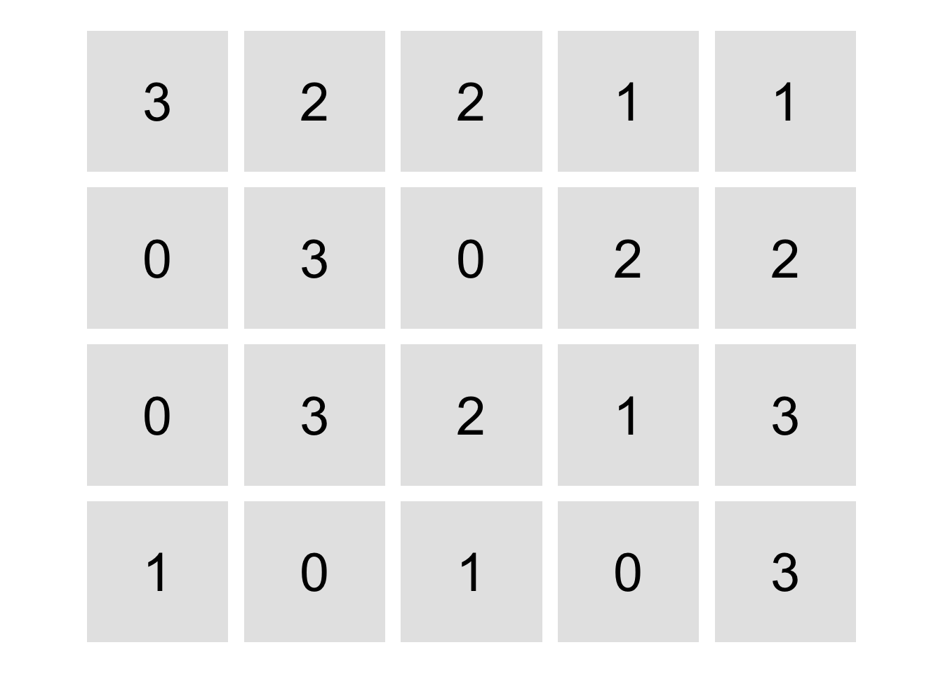
sol <- solve_dominosa(grid)
sol
row col direction
00 2 1 1
01 4 1 0
02 1 3 1
03 4 4 0
11 1 4 0
12 3 3 1
13 3 4 0
22 2 4 0
23 1 1 0
33 2 2 1create_dominosa_plot(grid, sol)
Larger Puzzle
Testing the solver works on a larger puzzle [clink the link to view an interactive version of the puzzle at Simon Tatham’s puzzle page]
grid <- matrix(c(
  5, 1, 6, 6, 3, 5, 0, 0,
  1, 6, 6, 6, 3, 6, 4, 2,
  1, 3, 4, 1, 3, 1, 2, 3,
  0, 5, 2, 2, 1, 4, 4, 1,
  0, 5, 4, 3, 4, 2, 2, 0,
  0, 4, 5, 3, 0, 6, 5, 0,
  5, 3, 2, 1, 4, 2, 5, 6
), nrow = 7, byrow = TRUE)

create_dominosa_plot(grid)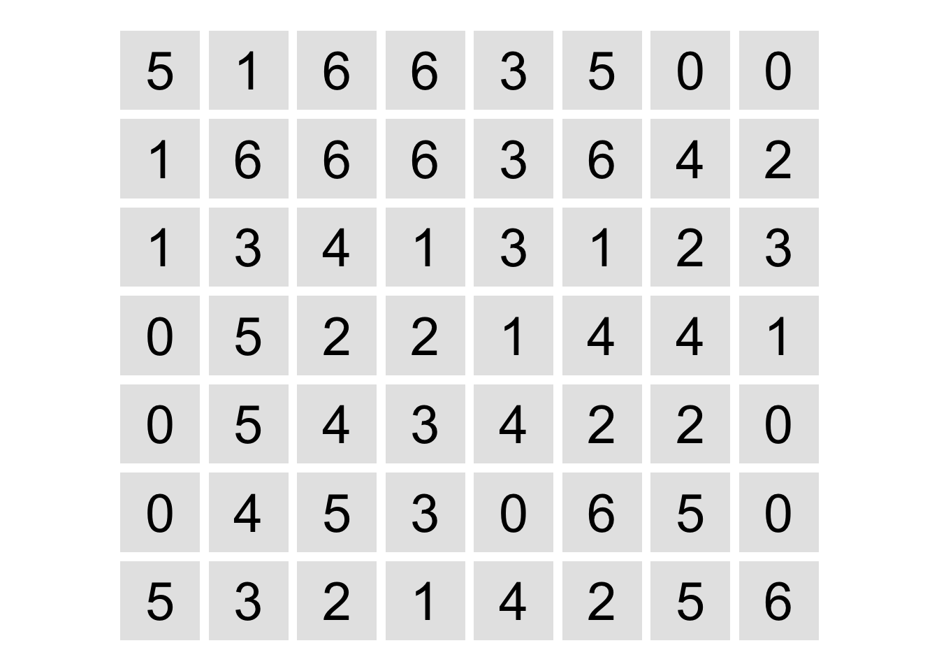
sol <- solve_dominosa(grid)

create_dominosa_plot(grid, sol)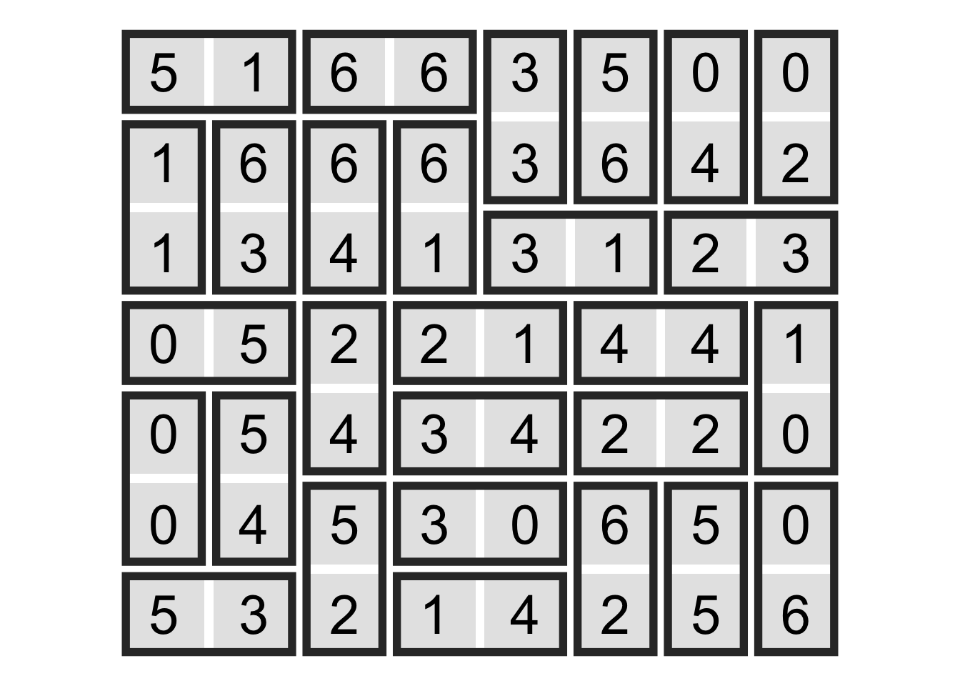
Summary
A fun exercise in recursive backtracking.
Appendix: plot_dominosa()
#~~~~~~~~~~~~~~~~~~~~~~~~~~~~~~~~~~~~~~~~~~~~~~~~~~~~~~~~~~~~~~~~~~~~~~~~~~~~~
#' Create a plot of a dominosa grid and solution
#'
#' @param grid Puzzle grid (matrix)
#' @param sol Solution matrix
#'
#' @return ggplot object
#~~~~~~~~~~~~~~~~~~~~~~~~~~~~~~~~~~~~~~~~~~~~~~~~~~~~~~~~~~~~~~~~~~~~~~~~~~~~~
create_dominosa_plot <- function(grid, sol = NULL) {
  grid_df <- tibble(
    value =  c(grid),
    row   = rep(seq(nrow(grid)), ncol(grid)),
    col   = rep(seq(ncol(grid)), each = nrow(grid))
  )

  grid_df <- grid_df %>% mutate(
    row   = max(row) + 1L - row
  )

  p <- ggplot(grid_df) +
    geom_tile(aes(col, row), width = 0.9, height = 0.9, fill = 'grey90') +
    geom_text(aes(col, row, label = value)) +
    theme_void() +
    coord_equal()

  if (!is.null(sol)) {
    sol_df <- as.tbl(as.data.frame(sol)) %>%
      mutate(
        row     = max(row) + 1L - row,
        row_end = if_else(direction == 1, row - 1L, row),
        col_end = if_else(direction == 0, col + 1L, col)
      ) %>% mutate(
        col      = col     - 0.42,
        row      = row     + 0.42,
        col_end  = col_end + 0.42,
        row_end  = row_end - 0.42
      )

    p <- p + geom_rect(data = sol_df, aes(xmin = col, xmax = col_end, ymin = row, ymax = row_end),
                       fill = NA, colour = 'grey20', size = 2)
  }

  p
}