Why the Hell would you do this?
Polygon filling is ubiquitous in computer graphics, with modern GPU hardware rendering approximately 1 Billion polygons per second.
So why have I regressed to 30 years ago and hand-rolled a scanline polygon filling algorithm in plain R?
- I needed it
- I hadn’t written one since Computer Graphics 101 - so many years ago.
- I was interested to see how much the built-in R data structures would help - mainly the use of data.frames to hold the edge lists.
Specifications
Specifications for my use case
- Base R only - I don’t want to compile C code or pull in some other dependency.
- Integer coordinates only. Everything will be rounded to an integer as I’m not anti-aliasing or anything fancy.
- Polygons only expected to be a maximum of about 100x100 pixels, so speed won’t be a huge factor.
Scanline Polygon Fill
See wikipedia for an overview of scanline rendering.
The code here is broken in to 2 functions:
make_edges()creates edge information for each pair of vertices in the polygonfill_polygon()fills the polygon specified by vectors of vertices.
#~~~~~~~~~~~~~~~~~~~~~~~~~~~~~~~~~~~~~~~~~~~~~~~~~~~~~~~~~~~~~~~~~~~~~~~~~~~~~
#' Make edge information structure from polygon vertex coords
#'
#' @param xs,ys vertex coords
#'
#' @return data.frame
#'
#' @importFrom utils head tail
#~~~~~~~~~~~~~~~~~~~~~~~~~~~~~~~~~~~~~~~~~~~~~~~~~~~~~~~~~~~~~~~~~~~~~~~~~~~~~
make_edges <- function(xs, ys) {

  #~~~~~~~~~~~~~~~~~~~~~~~~~~~~~~~~~~~~~~~~~~~~~~~~~~~~~~~~~~~~~~~~~~~~~~~~~~~
  # Ensure we have a closed loop
  #~~~~~~~~~~~~~~~~~~~~~~~~~~~~~~~~~~~~~~~~~~~~~~~~~~~~~~~~~~~~~~~~~~~~~~~~~~~
  N <- length(xs)
  if (!(xs[1] == xs[N] && ys[1] == ys[N])) {
    xs <- c(xs, xs[1])
    ys <- c(ys, ys[1])
  }

  #~~~~~~~~~~~~~~~~~~~~~~~~~~~~~~~~~~~~~~~~~~~~~~~~~~~~~~~~~~~~~~~~~~~~~~~~~~~
  # Basic edge structure: the 2 vertices
  #~~~~~~~~~~~~~~~~~~~~~~~~~~~~~~~~~~~~~~~~~~~~~~~~~~~~~~~~~~~~~~~~~~~~~~~~~~~
  edges <- data.frame(
    x1 = head(xs, -1),
    y1 = head(ys, -1),
    x2 = tail(xs, -1),
    y2 = tail(ys, -1)
  )

  #~~~~~~~~~~~~~~~~~~~~~~~~~~~~~~~~~~~~~~~~~~~~~~~~~~~~~~~~~~~~~~~~~~~~~~~~~~~
  # Enhanced edge structure
  #  - ymin,ymax the extents of this edge
  #  - x the x coordinate of ymin
  #  - igrad inverse gradient (used to increment the x as we step through the
  #          y scanlines)
  #~~~~~~~~~~~~~~~~~~~~~~~~~~~~~~~~~~~~~~~~~~~~~~~~~~~~~~~~~~~~~~~~~~~~~~~~~~~
  edges <- transform(
    edges,
    ymin  = pmin(y1, y2),
    ymax  = pmax(y1, y2),
    x     = ifelse(y2 > y1, x1, x2),
    igrad = (x2 - x1)/(y2 - y1)
  )

  #~~~~~~~~~~~~~~~~~~~~~~~~~~~~~~~~~~~~~~~~~~~~~~~~~~~~~~~~~~~~~~~~~~~~~~~~~~~
  # order by increasing ymin
  #~~~~~~~~~~~~~~~~~~~~~~~~~~~~~~~~~~~~~~~~~~~~~~~~~~~~~~~~~~~~~~~~~~~~~~~~~~~
  edges <- edges[order(edges$ymin),]

  edges
}
#~~~~~~~~~~~~~~~~~~~~~~~~~~~~~~~~~~~~~~~~~~~~~~~~~~~~~~~~~~~~~~~~~~~~~~~~~~~~~
#' Fill a polygon
#'
#' @param mat matrix to fill
#' @param xs,ys coordinates of vertices (integers)
#' @param fill fill value. usually a character.
#~~~~~~~~~~~~~~~~~~~~~~~~~~~~~~~~~~~~~~~~~~~~~~~~~~~~~~~~~~~~~~~~~~~~~~~~~~~~~
fill_polygon <- function(mat, xs, ys, fill) {
#~~~~~~~~~~~~~~~~~~~~~~~~~~~~~~~~~~~~~~~~~~~~~~~~~~~~~~~~~~~~~~~~~~~~~~~~~~~
# Ensure we only have integers
#~~~~~~~~~~~~~~~~~~~~~~~~~~~~~~~~~~~~~~~~~~~~~~~~~~~~~~~~~~~~~~~~~~~~~~~~~~~
xs <- round(as.integer(xs))
ys <- round(as.integer(ys))
stopifnot(length(xs) == length(ys))
#~~~~~~~~~~~~~~~~~~~~~~~~~~~~~~~~~~~~~~~~~~~~~~~~~~~~~~~~~~~~~~~~~~~~~~~~~~~
# Initialise the edge lists
#~~~~~~~~~~~~~~~~~~~~~~~~~~~~~~~~~~~~~~~~~~~~~~~~~~~~~~~~~~~~~~~~~~~~~~~~~~~
all_edges <- make_edges(xs, ys)
active <- NULL
if (nrow(all_edges) < 3) {
return(mat)
}
#~~~~~~~~~~~~~~~~~~~~~~~~~~~~~~~~~~~~~~~~~~~~~~~~~~~~~~~~~~~~~~~~~~~~~~~~~~~
# Set the vertices
#~~~~~~~~~~~~~~~~~~~~~~~~~~~~~~~~~~~~~~~~~~~~~~~~~~~~~~~~~~~~~~~~~~~~~~~~~~~
mat[cbind(ys, xs)] <- fill
#~~~~~~~~~~~~~~~~~~~~~~~~~~~~~~~~~~~~~~~~~~~~~~~~~~~~~~~~~~~~~~~~~~~~~~~~~~~
# Draw any horizontal edges and remove from list
#~~~~~~~~~~~~~~~~~~~~~~~~~~~~~~~~~~~~~~~~~~~~~~~~~~~~~~~~~~~~~~~~~~~~~~~~~~~
hedges <- subset(all_edges, y1 == y2)
all_edges <- subset(all_edges, y1 != y2)
for (i in seq_len(nrow(hedges))) {
hedge_row <- hedges[i, ]
ys <- hedge_row$y1
xs <- hedge_row$x1:hedge_row$x2
mat[ys, xs] <- fill
}
#~~~~~~~~~~~~~~~~~~~~~~~~~~~~~~~~~~~~~~~~~~~~~~~~~~~~~~~~~~~~~~~~~~~~~~~~~~~
# For each 'y' scanline
#~~~~~~~~~~~~~~~~~~~~~~~~~~~~~~~~~~~~~~~~~~~~~~~~~~~~~~~~~~~~~~~~~~~~~~~~~~~
for (yscan in min(all_edges$ymin):max(all_edges$ymax)) {
#~~~~~~~~~~~~~~~~~~~~~~~~~~~~~~~~~~~~~~~~~~~~~~~~~~~~~~~~~~~~~~~~~~~~~~~~~~~~~
# Add new active edges to 'active', and remove from 'all_edges'
#~~~~~~~~~~~~~~~~~~~~~~~~~~~~~~~~~~~~~~~~~~~~~~~~~~~~~~~~~~~~~~~~~~~~~~~~~~~~~
new_active <- subset(all_edges, ymin == yscan)
all_edges <- subset(all_edges, ymin > yscan)
active <- rbind(active, new_active)
#~~~~~~~~~~~~~~~~~~~~~~~~~~~~~~~~~~~~~~~~~~~~~~~~~~~~~~~~~~~~~~~~~~~~~~~~~~~~~
# Remove any active edges which the scanline has passed.
#~~~~~~~~~~~~~~~~~~~~~~~~~~~~~~~~~~~~~~~~~~~~~~~~~~~~~~~~~~~~~~~~~~~~~~~~~~~~~
active <- subset(active, ymax > yscan)
#~~~~~~~~~~~~~~~~~~~~~~~~~~~~~~~~~~~~~~~~~~~~~~~~~~~~~~~~~~~~~~~~~~~~~~~~~~~~~
# Check if all edges have been processed
#~~~~~~~~~~~~~~~~~~~~~~~~~~~~~~~~~~~~~~~~~~~~~~~~~~~~~~~~~~~~~~~~~~~~~~~~~~~~~
if (nrow(all_edges) == 0 && nrow(active) == 0) {
break
}
#~~~~~~~~~~~~~~~~~~~~~~~~~~~~~~~~~~~~~~~~~~~~~~~~~~~~~~~~~~~~~~~~~~~~~~~~~~~~~
# Arrange active list by x
#~~~~~~~~~~~~~~~~~~~~~~~~~~~~~~~~~~~~~~~~~~~~~~~~~~~~~~~~~~~~~~~~~~~~~~~~~~~~~
active <- active[order(active$x),]
#~~~~~~~~~~~~~~~~~~~~~~~~~~~~~~~~~~~~~~~~~~~~~~~~~~~~~~~~~~~~~~~~~~~~~~~~~~~~~
# For each pair of edges, draw the scanline between them
#~~~~~~~~~~~~~~~~~~~~~~~~~~~~~~~~~~~~~~~~~~~~~~~~~~~~~~~~~~~~~~~~~~~~~~~~~~~~~
for (pidx in seq(1, nrow(active), by=2)) {
x1 <- as.integer(round(active$x[pidx ]))
x2 <- as.integer(round(active$x[pidx + 1]))
ys <- yscan
xs <- x1:x2
mat[ys, xs] <- fill
}
#~~~~~~~~~~~~~~~~~~~~~~~~~~~~~~~~~~~~~~~~~~~~~~~~~~~~~~~~~~~~~~~~~~~~~~~~~~~~~
# Increment the x position of the active edges
#~~~~~~~~~~~~~~~~~~~~~~~~~~~~~~~~~~~~~~~~~~~~~~~~~~~~~~~~~~~~~~~~~~~~~~~~~~~~~
active$x <- active$x + active$igrad
}
mat
}Draw a filled hexagon in ASCII
#~~~~~~~~~~~~~~~~~~~~~~~~~~~~~~~~~~~~~~~~~~~~~~~~~~~~~~~~~~~~~~~~~~~~~~~~~~~~~
# Create a hexagon.  Distort in the x axis for better visual appearance since
# fonts are alwyas wider than they are tall.
#~~~~~~~~~~~~~~~~~~~~~~~~~~~~~~~~~~~~~~~~~~~~~~~~~~~~~~~~~~~~~~~~~~~~~~~~~~~~~
polygon_df <- tibble(
  angle = seq(0, 2*pi, length.out = 7) + pi/6,
  x     = 2.3 * (8 * cos(angle) + 11),
  y     = 8 * sin(angle) + 11
)


#~~~~~~~~~~~~~~~~~~~~~~~~~~~~~~~~~~~~~~~~~~~~~~~~~~~~~~~~~~~~~~~~~~~~~~~~~~~~~
# Initialise a blank matrix and draw the polygon on it.
#~~~~~~~~~~~~~~~~~~~~~~~~~~~~~~~~~~~~~~~~~~~~~~~~~~~~~~~~~~~~~~~~~~~~~~~~~~~~~
mat <- matrix('.', 20, 50)
mat <- fill_polygon(mat, xs = polygon_df$x, ys = polygon_df$y, fill = '#')

#~~~~~~~~~~~~~~~~~~~~~~~~~~~~~~~~~~~~~~~~~~~~~~~~~~~~~~~~~~~~~~~~~~~~~~~~~~~~~
# Add some text and dump the canvas to the console
#~~~~~~~~~~~~~~~~~~~~~~~~~~~~~~~~~~~~~~~~~~~~~~~~~~~~~~~~~~~~~~~~~~~~~~~~~~~~~
mat[11, 18:31] <- strsplit('Hello #RStats!', '')[[1]]
cat(apply(mat, 1, paste, collapse = ""), sep="\n")
..................................................
..................................................
........................#.........................
....................##########....................
................####################..............
............#############################.........
........#################################.........
........#################################.........
........#################################.........
........#################################.........
........#########Hello #RStats!##########.........
........#################################.........
........#################################.........
........#################################.........
........#################################.........
............#########################.............
................#################.................
....................#########.....................
........................#.........................
..................................................Drawing with ANSI
Instead of just ASCII characters, you would use ANSI colours to make something prettier. Here I’ll use ransid for the ANSI codes (but in general you will probably want to use something well-designed like crayon)
Note: ANSI colours won’t display in an Rmarkdown document (as far as I know), so I’ve just taken a screen capture of my terminal and included the image.
library(ransid)

#~~~~~~~~~~~~~~~~~~~~~~~~~~~~~~~~~~~~~~~~~~~~~~~~~~~~~~~~~~~~~~~~~~~~~~~~~~~~~
# Define some ANSI strings for the colours I want
#~~~~~~~~~~~~~~~~~~~~~~~~~~~~~~~~~~~~~~~~~~~~~~~~~~~~~~~~~~~~~~~~~~~~~~~~~~~~~
dark_bg  <- paste0(col2bg('darkblue' ), ' ')
light_bg <- paste0(col2bg('lightblue'), ' ')
text_fg  <- paste0(col2fg('red'   ))
text_bg  <- paste0(col2bg('yellow'))

#~~~~~~~~~~~~~~~~~~~~~~~~~~~~~~~~~~~~~~~~~~~~~~~~~~~~~~~~~~~~~~~~~~~~~~~~~~~~~
# Initialise a matrix with a light background and draw the polygon on it.
#~~~~~~~~~~~~~~~~~~~~~~~~~~~~~~~~~~~~~~~~~~~~~~~~~~~~~~~~~~~~~~~~~~~~~~~~~~~~~
mat <- matrix(light_bg, 20, 50)
mat <- fill_polygon(mat, xs = polygon_df$x, ys = polygon_df$y, fill=dark_bg)

#~~~~~~~~~~~~~~~~~~~~~~~~~~~~~~~~~~~~~~~~~~~~~~~~~~~~~~~~~~~~~~~~~~~~~~~~~~~~~
# Add some text and dump the canvas to the console
#~~~~~~~~~~~~~~~~~~~~~~~~~~~~~~~~~~~~~~~~~~~~~~~~~~~~~~~~~~~~~~~~~~~~~~~~~~~~~
mat[11, 18:31] <- paste0(text_fg, text_bg, strsplit('Hello #RStats!', '')[[1]])
res <- paste0(apply(mat, 1, paste, collapse = ""), collapse="\n")
cat(res)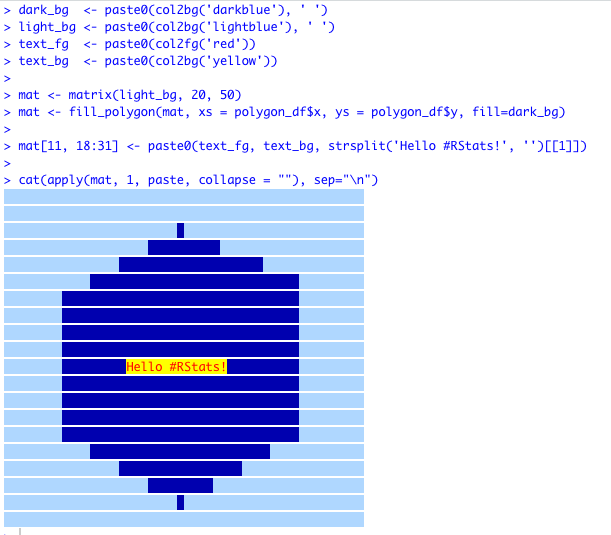
Animating the ANSI
Dump ANSI to the console and screencapture it to a gif. Inelegant, but it works for now.
#~~~~~~~~~~~~~~~~~~~~~~~~~~~~~~~~~~~~~~~~~~~~~~~~~~~~~~~~~~~~~~~~~~~~~~~~~~~~~
# Create a hexagon.  Distort in the x axis for better visual appearance since
# fonts are alwyas wider than they are tall.
#~~~~~~~~~~~~~~~~~~~~~~~~~~~~~~~~~~~~~~~~~~~~~~~~~~~~~~~~~~~~~~~~~~~~~~~~~~~~~
for (start_angle in seq(pi/6, pi/2, length.out = 30)) {
  polygon_df <- tibble(
    angle = seq(0, 2*pi, length.out = 7) + start_angle,
    x     = 2.3 * (16 * cos(angle) + 21),
    y     = 16 * sin(angle) + 21
  )


  #~~~~~~~~~~~~~~~~~~~~~~~~~~~~~~~~~~~~~~~~~~~~~~~~~~~~~~~~~~~~~~~~~~~~~~~~~~~~~
  # Initialise a matrix with a light background and draw the polygon on it.
  #~~~~~~~~~~~~~~~~~~~~~~~~~~~~~~~~~~~~~~~~~~~~~~~~~~~~~~~~~~~~~~~~~~~~~~~~~~~~~
  mat <- matrix(light_bg, 40, 100)
  mat <- fill_polygon(mat, xs = polygon_df$x, ys = polygon_df$y, fill=dark_bg)

  #~~~~~~~~~~~~~~~~~~~~~~~~~~~~~~~~~~~~~~~~~~~~~~~~~~~~~~~~~~~~~~~~~~~~~~~~~~~~~
  # Add some text and dump the canvas to the console
  #~~~~~~~~~~~~~~~~~~~~~~~~~~~~~~~~~~~~~~~~~~~~~~~~~~~~~~~~~~~~~~~~~~~~~~~~~~~~~
  mat[21, 41:54] <- paste0(text_fg, text_bg, strsplit('Hello #RStats!', '')[[1]])
  cat(paste0(apply(mat, 1, paste, collapse = ""), sep="\n"))
  Sys.sleep(0.3)
}