Introduction

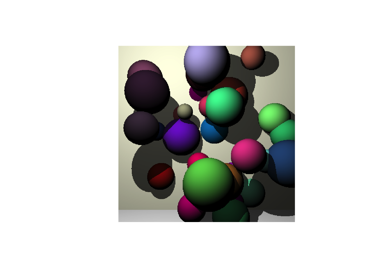
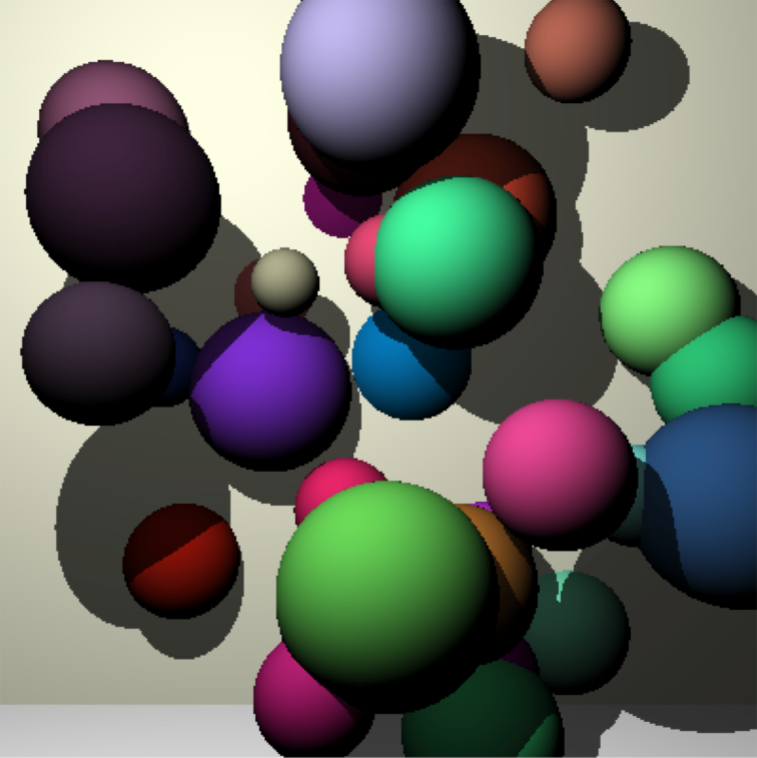
This code was a personal challenge to write a simple ray-tracer in pure R.

Ray tracing is an example of something which is really silly to do in base R, and I’d be interested to see how others would approach this problem.

Code is shared in a public gist. Please share and enjoy.

Design

Has to be base R only. No other packages allowed
Supports sphereical objects only. This simplifies object handling.
Tracing a single eye-ray per pixel only
Single light probe rays for shadow testing
Objects represented by signed distance fields.
Ray-marching/Sphere-tracing is used to move rays through space

Setting expectations

This is what Blender can do

This is what this code does

Data representation

rays - a bundle of rays stored as a list of matrices. Stores ray origin, direction, distance travelled so far, closest object index, distance to closest object
sphere - a list of information about a spherical object i.e. coordinates of centre, radius and colour

Helper functions

Normalise vectors `normalise()`

#-----------------------------------------------------------------------------
#' Normalise vectors to unit length
#' @param mat a matrix storing multiple vectors i.e. one vector per row
#' @return modified matrix with all vectors normalised to length=1
#-----------------------------------------------------------------------------
normalise <- function(mat) {
  mat / sqrt(rowSums(mat ^ 2))
}

Plot values associated with a bundle of rays - `draw()`

#-----------------------------------------------------------------------------
#' Draw a ray parameter shading with viridis
#' @param rays list of ray information
#' @param paramter valid ray parameter e.g. 't', 'obj_index', 'dist2obj'
#' @param ... other parameters passed to `viridisLit::viridis()`
#-----------------------------------------------------------------------------
draw <- function(rays, parameter, option = 'A', ...) {
  values <- rays[[parameter]]

  if (length(unique(values)) == 1) {
    values[] <- 0
  } else {
    values <- as.integer(255 * (values - min(values)) / (max(values) - min(values)))
  }

  colours <- viridisLite::viridis(256, option = option, ...)[values + 1L]
  mat <- matrix(colours, N, N)
  mat <- mat[rev(seq(N)),]

  plot(as.raster(mat), interpolate = FALSE)
}

Create rays through image plane - `create_eye_rays()`

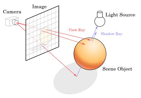
Eye rays are the rays which are cast from the eye through each pixel in the screen.

The colour of the object at the end of this ray is the colour of the pixel in the final image representation.

An illustration of these rays is included below:

#-----------------------------------------------------------------------------
#' Create the initial set of eye rays
#' Image plane is in the x,y plane centered at c(0, 0, 0)
#' @param N pixel width and height of the resulting image
#' @param eye_to_image_plane default: 2
#-----------------------------------------------------------------------------
create_eye_rays <- function(N=5, eye_to_image_plane = 2) {
  eye <- c(0, 0, -eye_to_image_plane)
  mid <- as.integer((N+1)/2)

  col <- rep(1:N, each=N)
  row <- rep(1:N,      N)

  x <- (col - mid) / (mid - 1)
  y <- (row - mid) / (mid - 1)

  ray_origin  <- cbind(x=x, y=y, z=0)

  ray_dir <- ray_origin
  ray_dir[,1] <- ray_origin[,1] - eye[1]
  ray_dir[,2] <- ray_origin[,2] - eye[2]
  ray_dir[,3] <- ray_origin[,3] - eye[3]

  ray_dir <- normalise(ray_dir)

  rays <- list(
    origin    = ray_origin,
    dir       = ray_dir,
    t         = numeric(N*N),
    obj_index = NA,
    steps     = rep(-1L, N*N)
  )

  rays$ray_end <- rays$origin + rays$dir * rays$t

  rays
}

Signed distance function - `calc_distances_to_sphere()`

This renderer uses signed distance functions to determine the distance from the position of any point in space to a given object.

Each ray is tested against each object. The distance to the closet object determines how far the ray will advance at the next time step (and be guaranteed to not hit anything else). This is ray-marching with sphere-tracing.

#-----------------------------------------------------------------------------
#' Core function to calculate distance from sphere and a bundle of rays
#-----------------------------------------------------------------------------
calc_distances_to_sphere <- function(sphere, rays) {
  sqrt(colSums( (t(rays$ray_end) - sphere$centre) ^ 2 )) - sphere$radius
}

Ray marching - `raymarch()`

This function orchestrates the marching of a bundle of rays within a scene containing a set of objects.

It proceeds as follows:

For each ray, find the distance to the nearest object
Advance the ray that distance
Repeat.

The sphere-tracing/ray-marching step is illustrated in the figure below (from hasmcole.com)

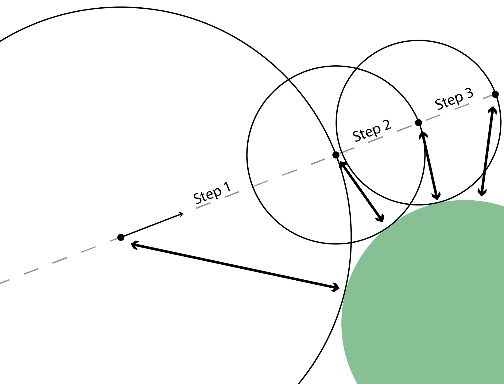
Note: There is no convergence criteria used here to determine if a ray has actually hit an object. Instead, all rays are marched through the scene a fixed number of times. This is pretty naive, and there would be speed gains by stopping the marching of rays which have already intersected an object.

#-----------------------------------------------------------------------------
#' march the rays
#-----------------------------------------------------------------------------
raymarch <- function(rays, objects) {

  #---------------------------------------------------------------------------
  # Naive marching. Just goint to a fixed number of iterations
  #  1. Calc distance from end of each ray to the nearest object
  #  2. Ray march (sphere tracing) to advance the ray this minimum distance
  #  3. Repeat
  #---------------------------------------------------------------------------
  for (step in seq_len(100)) {
    distances      <- lapply(objects, calc_distances_to_sphere, rays)
    rays$dist2obj  <- do.call(pmin.int, distances)
    rays$t         <- rays$t + rays$dist2obj
    rays$ray_end   <- rays$origin + rays$dir * rays$t
    
    # Keep a rough notion of the step number at which the ray converged 
    # on an object
    just_converged <- rays$dist2obj < 0.001 & rays$step < 0
    rays$step[just_converged] <- step
  }

  #---------------------------------------------------------------------------
  # Ray cleanup
  #  - find closest object
  #  - mark objects within a given idstance as 'converged'
  #---------------------------------------------------------------------------
  rays$obj_index <- max.col(-do.call(cbind, distances))
  rays$converged <- rays$dist2obj < 0.01
  rays$step[rays$step < 0] <- step

  rays
}

Define the objects in the scene

Only spheres are supported, with each object represented as a list of centre, radius and colour.

The back wall and floor are just very large spheres.

The specifications for the spheres is also stored as matrices to ease the creation of light probe rays and colour calculations.

#-----------------------------------------------------------------------------
#' Place some random spheres
#-----------------------------------------------------------------------------
set.seed(1)
random_spheres <- lapply(1:35, function(x) {
  radius <- runif(1, 0.2, 0.8)
  x      <- runif(1,  -3, 3)
  y      <- runif(1,  -3, 3)
  z      <- runif(1, 3, 6) #- radius
  list(centre = c(x, y, z), radius = radius, colour = runif(3))
})

walls <- list(
  list(centre = c(0  ,    0  , 900), radius = 895  , colour = c(1, 1, 0.9)),  # back wall,
  list(centre = c(0  , -900  ,   0), radius = 897  , colour = c(1, 1, 1  ))   # floor
)

regular_objects <- c(random_spheres, walls)


#-----------------------------------------------------------------------------
# Extract summary representations across all objects of:
#  - colours
#  - centres
#  - radii
#-----------------------------------------------------------------------------
object_colours <- lapply(regular_objects, `[[`, 'colour')
object_colours <- do.call(rbind, object_colours)

object_radii <- vapply(regular_objects, `[[`, numeric(1), 'radius')

object_centres <- lapply(regular_objects, `[[`, 'centre')
object_centres <- do.call(rbind, object_centres)

Render the scene

Create rays from the eye through each pixel in the output image
March these rays through the scene, using the sphere objects to define how far to advance at each step

#-----------------------------------------------------------------------------
#' Create a bundle of NxN rays and march them into the scene
#-----------------------------------------------------------------------------
N <- 400
eye_rays <- create_eye_rays(N)

print(system.time({
  rays <- raymarch(eye_rays, regular_objects)
}))

##    user  system elapsed 
##  20.802   4.282  25.126

Information about the render

Each ray retains some information about how it travelled through the scene:

The index of the closest object - obj_index
The number of steps to converge on an object - step
The distance travelled - t

draw(rays, 'obj_index'); title("Index of object closest to end of eye ray")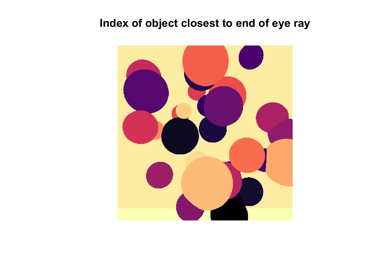

draw(rays, 't')        ; title("Distance ray has travelled")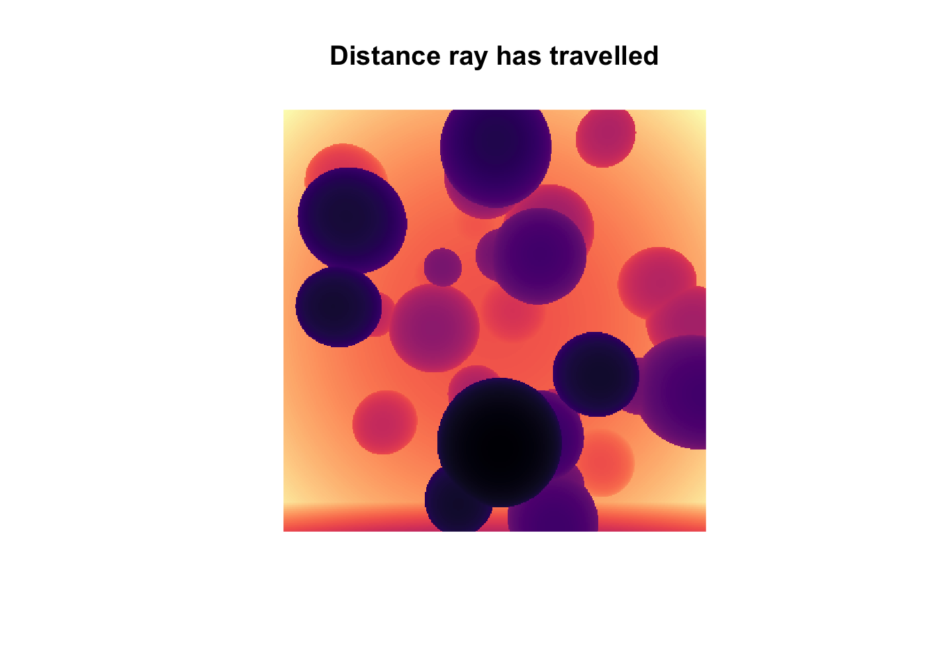

draw(rays, 'step')     ; title("Number of steps to converge")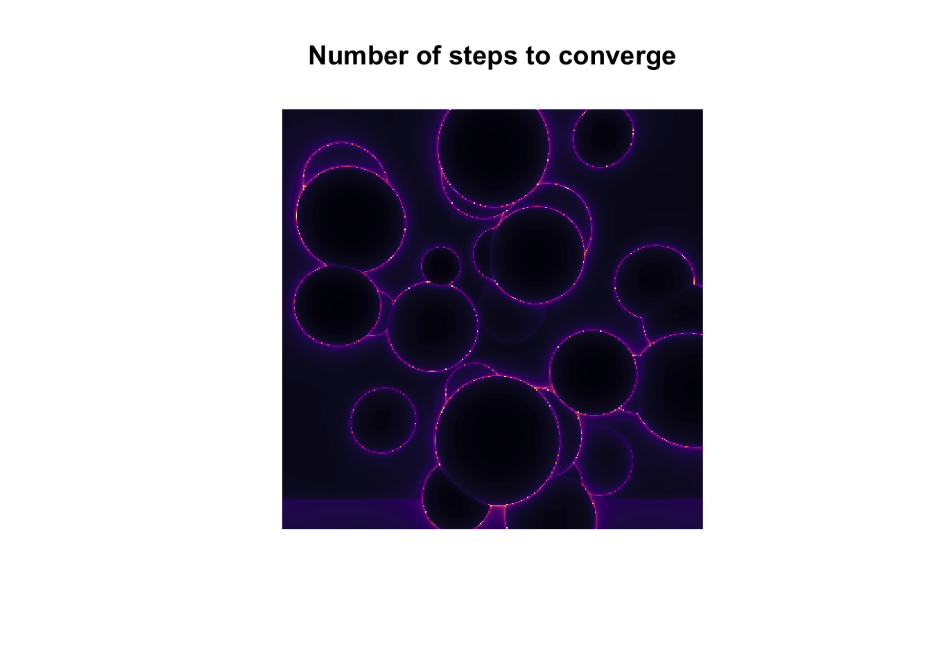

This last image is interesting as it shows that rays which pass near to the edge of an object takes more steps to converge.

As illustrated below, this is because as a ray grazes an object it takes a large number of very small steps.

Shadows

To determine which objects are in light and which are in shadow:

Define a light source object
At the end of each ray, determine the local surface normal and direction to this light source
Ray march these new light probe rays
If they hit the light, then it means there are no objects in the way and it is fully lit. Otherwise it is in shadow

#-----------------------------------------------------------------------------
# Define the position of the light within the scene
#-----------------------------------------------------------------------------
light <- list(centre=c(-1.5, 2.5, 0.2), radius=0.1)


#-----------------------------------------------------------------------------
# Calculate probes from the end of each camera ray to the light source.
#  (1) find object each ray intersects
#  (2) Find the centre of this object and the local normal
#  (3) Calculate the direction from this intersection to the light source
#  (4) Construct set of rays to probe for visibilit of light source
#-----------------------------------------------------------------------------
centres <- object_centres[rays$obj_index,]

normal <- rays$ray_end - centres
normal <- normalise(normal)

radii <- object_radii[rays$obj_index]

# Start light ray from just above surface
intersect <- centres + (radii + 0.001) * normal

# Direction to lightsource (normalised to unit length)
dir <- intersect
dir[,1] <- light$centre[1] - intersect[,1]
dir[,2] <- light$centre[2] - intersect[,2]
dir[,3] <- light$centre[3] - intersect[,3]
dir <- normalise(dir)

# Dot product of local normal with direction to lightsource.
# Clamp negative values (where normal points away from light) to zero
facing_light <- (dir[,1]*normal[,1] + dir[,2]*normal[,2] + dir[,3]*normal[,3])
facing_light <- ifelse(facing_light > 0, facing_light, 0)

# Construct light probes
light_probes <- list(
  origin = intersect,
  dir    = dir,
  t      = numeric(length(radii))
)

light_probes$ray_end <- light_probes$origin + light_probes$dir * light_probes$t


#-----------------------------------------------------------------------------
#' raymarch the light probes
#' If a lightprobe hits the light, then the object can see the light source,
#' otherwise it is in shadow
#-----------------------------------------------------------------------------
objects_with_light <- c(list(light), regular_objects)
light_probes       <- raymarch(light_probes, objects_with_light)

Determine colour and shading of each pixel

#-----------------------------------------------------------------------------
# Find the colour of each object at the end of each eye ray
# If ray is not close to any object, set colour to black
#-----------------------------------------------------------------------------
intersect_colour <- object_colours[rays$obj_index,]
intersect_colour[rays$dist2obj > 0.1, ] <- 0

#-----------------------------------------------------------------------------
# If a light probe from this intersection intersects with any object other
# than the light source, then it is in shadow, so darken this colour
#-----------------------------------------------------------------------------
in_shadow <- light_probes$obj_index != 1
intersect_colour[in_shadow] <- 0.3 * intersect_colour[in_shadow]

#-----------------------------------------------------------------------------
# Shade the colour from light-to-dark depending on how close the local normal
# aligns with the direction of the light source.
#-----------------------------------------------------------------------------
final_colour <- intersect_colour * facing_light


#-----------------------------------------------------------------------------
# Convert final colours to a raster for plotting
#-----------------------------------------------------------------------------
colours <- rgb(final_colour[,1], final_colour[,2], final_colour[,3])
image   <- matrix(colours, nrow = N, ncol = N)
image   <- image[rev(seq(nrow(image))),] # flip top-to-bottom
image   <- as.raster(image)

plot(image, interpolate = FALSE)

A Simple Ray-Tracer Written in Base R