ggsvg - Use SVG as points in ggplot

ggsvg is an extension to ggplot to use arbitrary SVG as points.

This SVG can be customised to respond to aesthetics e.g. element colours can changes in response to fill and/or colour scales.

However, aesthetics are not limited to colour - any other SVG parameter can be linked to any aesthetic which makes sense e.g. an aesthethic may be used to control the corner radius on a rounded rectangle.

What’s in the box

geom_point_svg() is equivalent to geom_point() except it also requires SVG text to be set (via the svg argument)
scale_svg_* a full(?) set of compatible scale functions for controlling the mapping of values to arbitrary named aesthetics.

Installation

You can install from GitHub with:

# install.package('remotes')
remotes::install_github('coolbutuseless/cssparser')
remotes::install_github('coolbutuseless/svgparser')
remotes::install_github('coolbutuseless/ggsvg')

Debugging

Set options(GGSVG_DEBUG = TRUE) for some verbose debugging.

This will cause {ggsvg} to output the final SVG for each and every element it wants to put on the plot.

Simple SVG Image

An SVG Christmas Tree with a hex star on top!

library(ggplot2)
library(ggsvg)

#~~~~~~~~~~~~~~~~~~~~~~~~~~~~~~~~~~~~~~~~~~~~~~~~~~~~~~~~~~~~~~~~~~~~~~~~~~
# Define simple SVG
#   - Square with rounded corners and a circle inside it.
#~~~~~~~~~~~~~~~~~~~~~~~~~~~~~~~~~~~~~~~~~~~~~~~~~~~~~~~~~~~~~~~~~~~~~~~~~~
svg_text <- '
  <svg viewBox="0 0 100 100 ">
    <polygon points = "20,80 80,80 50,20" fill="darkgreen" />
    <polygon points = "40,83 60,83 60,95 40,95" fill="darkred" />
    <polygon points = "58.66 25.00 50.00 30.00 41.34 25.00 41.34 15.00 50.00 10.00 58.66 15.00 58.66 25.00" 
       fill="yellow3" />
  </svg>
  '


#~~~~~~~~~~~~~~~~~~~~~~~~~~~~~~~~~~~~~~~~~~~~~~~~~~~~~~~~~~~~~~~~~~~~~~~~~~
# Render SVG with `{svgparser}`
#~~~~~~~~~~~~~~~~~~~~~~~~~~~~~~~~~~~~~~~~~~~~~~~~~~~~~~~~~~~~~~~~~~~~~~~~~~
grob <- svgparser::read_svg(svg_text)
grid::grid.newpage()
grid::grid.draw(grob)

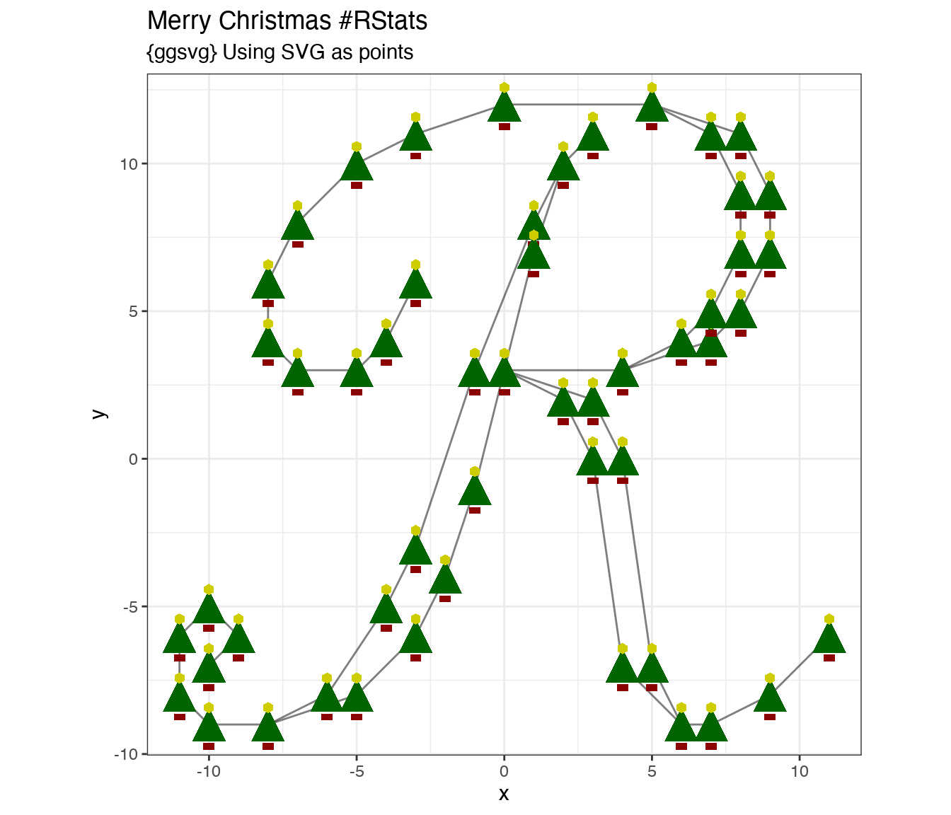
Simple SVG drawn for each point

Here, the simple SVG will be used as a plotting character.

The point locations are given by the capital “R” in the Hershey script font.

# remotes::install_github('coolbutuseless/hershey')
library(hershey)
letter <- hershey[hershey$char == 'R' & hershey$font == 'scriptc',]

#~~~~~~~~~~~~~~~~~~~~~~~~~~~~~~~~~~~~~~~~~~~~~~~~~~~~~~~~~~~~~~~~~~~~~~~~~~
# Use 'geom_point_svg' to plot SVG image at each point
#~~~~~~~~~~~~~~~~~~~~~~~~~~~~~~~~~~~~~~~~~~~~~~~~~~~~~~~~~~~~~~~~~~~~~~~~~~
ggplot(letter) +
  geom_path(aes(x, y, group = stroke), alpha = 0.5) +
  geom_point_svg(
    mapping  = aes(x, y),
    svg      = svg_text,
    size     = 10
  ) +
  theme_bw() + 
  coord_equal() + 
  labs(
    title    = "Merry Christmas #RStats",
    subtitle = "{ggsvg} Using SVG as points"
  )

Simple aesthetics

This is a basic example showing how ggplot aesthetics may be used to control SVG image properties.

Some key things to note:

Locations for ggplot to insert aesthetics via the glue package are marked with double curly braces i.e. {{...}}.
One such variables has been added to the SVG - {{fill_tree}} is used in place of the static colour that was defined in the original SVG
fill_tree must now appear as an aesthetic in the call to geom_point_svg()
Need to inform ggplot2 of the default value for each new aesthetic by setting the defaults argument
For each aesthetic, you will need to add a scale with scale_svg_*() to let ggplot know how it should turn the mapped variable into a value to insert in the SVG.
In this case, the variables is a fill variable, so use one of scale_svg_fill_*() family to ensure that the value is mapped to a colour.
The new scale_svg_*() scales are mostly identical to their ggplot counterparts except:
- The aesthetics argument no longer has a default value
- colourbar guides have been tweaked to allow for non-standard aesthetics.

library(ggplot2)
library(ggsvg)

#~~~~~~~~~~~~~~~~~~~~~~~~~~~~~~~~~~~~~~~~~~~~~~~~~~~~~~~~~~~~~~~~~~~~~~~~~~
# Define some SVG
#~~~~~~~~~~~~~~~~~~~~~~~~~~~~~~~~~~~~~~~~~~~~~~~~~~~~~~~~~~~~~~~~~~~~~~~~~~
svg_text <- '
  <svg viewBox="0 0 100 100 ">
    <polygon points = "20,80 80,80 50,20" fill="{{fill_tree}}" />
    <polygon points = "40,83 60,83 60,95 40,95" fill="darkred" />
    <polygon points = "58.66 25.00 50.00 30.00 41.34 25.00 41.34 15.00 50.00 10.00 58.66 15.00 58.66 25.00" 
       fill="yellow3" />
  </svg>
  '

#~~~~~~~~~~~~~~~~~~~~~~~~~~~~~~~~~~~~~~~~~~~~~~~~~~~~~~~~~~~~~~~~~~~~~~~~~~
# Use 'geom_svg' to plot with this symbol
#~~~~~~~~~~~~~~~~~~~~~~~~~~~~~~~~~~~~~~~~~~~~~~~~~~~~~~~~~~~~~~~~~~~~~~~~~~
ggplot(mtcars) +
  geom_point_svg(
    mapping     = aes(
      x           = mpg, 
      y           = wt, 
      size        = cyl, 
      fill_tree   = as.factor(cyl)
    ),
    svg         = svg_text,
    defaults    = list(fill_tree = 'darkgreen')
  ) +
  labs(
    title    = "{ggsvg} Simple SVG with fill aesthetic",
    subtitle = "`cyl` mapped to tree colour and size"
  ) + 
  theme_bw() +
  scale_size(range = c(5, 12), guide = 'none') + 
  scale_svg_fill_viridis_d('fill_tree', guide = guide_legend(override.aes = list(size = 7)))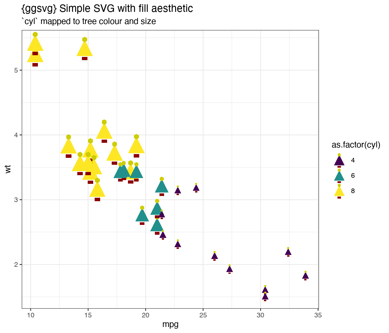

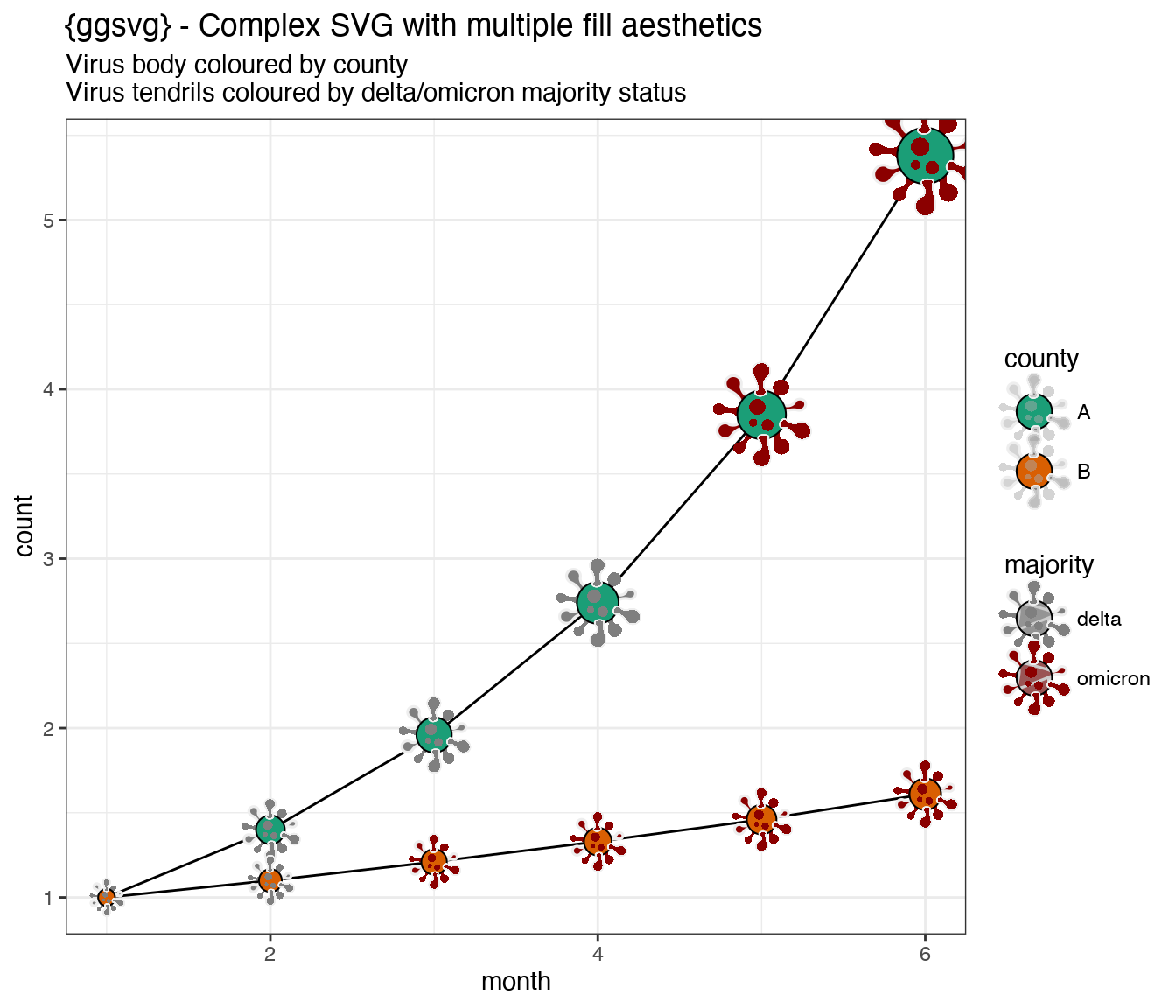
More complex example - Virus with multiple aesthetics

This is an SVG image of something virus-like from wikimedia - it is public domain.

svg_file <- system.file("Virus_black_white.svg", package = "ggsvg")
grob <- svgparser::read_svg(svg_file)
grid::grid.draw(grob)

I have hand-edited the SVG to add two locations for {glue} to insert text:

fill = "{{fill_inner}}" has been added to all elements in the central body of the virus.
fill = "{{fill_outer}}" has been added to the “arms” of the virus

library(ggplot2)
library(ggsvg)

fake_data <- readr::read_csv(
'county, month, count, majority
A, 1, 1.00, delta
A, 2, 1.40, delta
A, 3, 1.96, delta
A, 4, 2.74, delta
A, 5, 3.85, omicron
A, 6, 5.38, omicron
B, 1, 1.00, delta
B, 2, 1.10, delta
B, 3, 1.21, omicron
B, 4, 1.33, omicron
B, 5, 1.46, omicron
B, 6, 1.61, omicron
', show_col_types = FALSE)


#~~~~~~~~~~~~~~~~~~~~~~~~~~~~~~~~~~~~~~~~~~~~~~~~~~~~~~~~~~~~~~~~~~~~~~~~~~
# Read in the SVG as text.
#~~~~~~~~~~~~~~~~~~~~~~~~~~~~~~~~~~~~~~~~~~~~~~~~~~~~~~~~~~~~~~~~~~~~~~~~~~
svg_file <- system.file("virus.svg", package = "ggsvg")
svg_text <- paste(readLines(svg_file), collapse = "\n")

#~~~~~~~~~~~~~~~~~~~~~~~~~~~~~~~~~~~~~~~~~~~~~~~~~~~~~~~~~~~~~~~~~~~~~~~~~~
# Use 'geom_svg' to plot with this symbol
#~~~~~~~~~~~~~~~~~~~~~~~~~~~~~~~~~~~~~~~~~~~~~~~~~~~~~~~~~~~~~~~~~~~~~~~~~~
ggplot(fake_data) +
  geom_line(aes(month, count, group = county)) +
  geom_point_svg(
    mapping = aes(month, count, 
                  size = count, 
                  fill_inner = county, 
                  fill_outer = majority),
    svg         = svg_text,
    defaults    = list(fill_inner = '#aaaaaa80', fill_outer = '#aaaaaa80')
  ) +
  theme_bw() +
  scale_size_continuous(range = c(6, 20), guide = 'none') +
  scale_svg_fill_brewer(
    aesthetics = 'fill_inner', 
    palette = 'Dark2',
    guide = guide_legend(override.aes = list(size = 9))
  ) +
  scale_svg_fill_manual(
    aesthetics = 'fill_outer',
    values = c(delta = 'grey50', omicron = 'darkred'),
    guide = guide_legend(override.aes = list(size = 9))
  ) + 
  labs(
    title    = "{ggsvg} - Complex SVG with multiple fill aesthetics",
    subtitle = "Virus body coloured by county\nVirus tendrils coloured by delta/omicron majority status"
  )

Acknowledgements

R Core for developing and maintaining the language.
CRAN maintainers, for patiently shepherding packages onto CRAN and maintaining the repository

Introducing {ggsvg} - use SVG as ggplot points