Barnsley fern via iterated affine transformations (matrix ops)
Today in my ongoing quest to generate fractals in Rstats using every available avenue: generating Barnsley ferns via iterated affine transformations (matrix ops)
Methods for generating fractals so far:
- Sierpinski Triangle in plotmath
- Another sierpinski triangle in plotmath
- Sierpinski triangle using character strings
- Using R matrices to create a sierpinski carpet
- Generating hilbert curves with an ad-hoc L-system
- Today: Barnsley fern generated by iterated affine transformations
Barnsley ferns
Barnsley ferns are fractals generated by an iterated function system.
Generation of the fractal consists of just 2 repeated steps:
- Randomly choose an affine transformation from a set of transformations.
- Apply the transformation to the current point to find the next point.
#~~~~~~~~~~~~~~~~~~~~~~~~~~~~~~~~~~~~~~~~~~~~~~~~~~~~~~~~~~~~~~~~~~~~~~~~~~~~~
# 4 Transformations i.e. p(n+1) = A * p(n) + a
#~~~~~~~~~~~~~~~~~~~~~~~~~~~~~~~~~~~~~~~~~~~~~~~~~~~~~~~~~~~~~~~~~~~~~~~~~~~~~
A <- matrix(c( 0   ,  0   ,  0   , 0.16), nrow=2); a = c(0, 0.00); pa = 0.01
B <- matrix(c( 0.85, -0.04,  0.04, 0.85), nrow=2); b = c(0, 1.60); pb = 0.85
C <- matrix(c( 0.20,  0.23, -0.26, 0.22), nrow=2); c = c(0, 1.60); pc = 0.07
D <- matrix(c(-0.15,  0.26,  0.28, 0.24), nrow=2); d = c(0, 0.44); pd = 0.07
K <- list(A, B, C, D)
k <- list(a, b, c, d)

#~~~~~~~~~~~~~~~~~~~~~~~~~~~~~~~~~~~~~~~~~~~~~~~~~~~~~~~~~~~~~~~~~~~~~~~~~~~~~
# Each iteration produces a single point
#~~~~~~~~~~~~~~~~~~~~~~~~~~~~~~~~~~~~~~~~~~~~~~~~~~~~~~~~~~~~~~~~~~~~~~~~~~~~~
N <- 100000

#~~~~~~~~~~~~~~~~~~~~~~~~~~~~~~~~~~~~~~~~~~~~~~~~~~~~~~~~~~~~~~~~~~~~~~~~~~~~~
# Each iteration uses a randomly selected transformation
#~~~~~~~~~~~~~~~~~~~~~~~~~~~~~~~~~~~~~~~~~~~~~~~~~~~~~~~~~~~~~~~~~~~~~~~~~~~~~
s <- sample(1:4, N, prob = c(pa, pb, pc, pd), replace = TRUE)

#~~~~~~~~~~~~~~~~~~~~~~~~~~~~~~~~~~~~~~~~~~~~~~~~~~~~~~~~~~~~~~~~~~~~~~~~~~~~~
# Allocate space for the iterated points
#~~~~~~~~~~~~~~~~~~~~~~~~~~~~~~~~~~~~~~~~~~~~~~~~~~~~~~~~~~~~~~~~~~~~~~~~~~~~~
P <- matrix(0, nrow=2, ncol=N+1)
for (i in seq(N)) {
  M = K[[s[i]]]
  m = k[[s[i]]]
  P[,i+1] = M %*% P[,i] + m
}

plot(P[1,], P[2,],as=1,pch='.',an=F,ax=F)
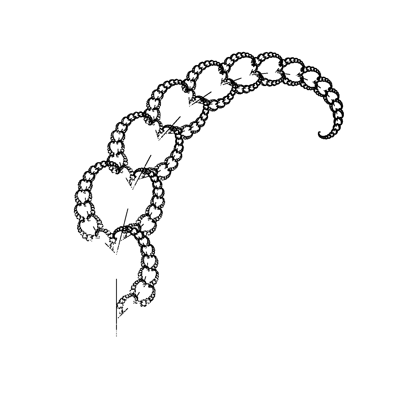
Mutant Varieties
By tweaking the affine transformations, new fern varieties can be created.
A <- matrix(c( 0    ,  0    ,  0    , 0.25),nr=2); a = c( 0    , -0.4 ); pa = 0.02
B <- matrix(c( 0.95 ,  0.005, -0.005, 0.93),nr=2); b = c(-0.002,  0.5 ); pb = 0.84
C <- matrix(c( 0.035, -0.2  ,  0.16 , 0.04),nr=2); c = c(-0.09 ,  0.02); pc = 0.07
D <- matrix(c(-0.04 ,  0.2  ,  0.16 , 0.04),nr=2); d = c( 0.083,  0.12); pd = 0.07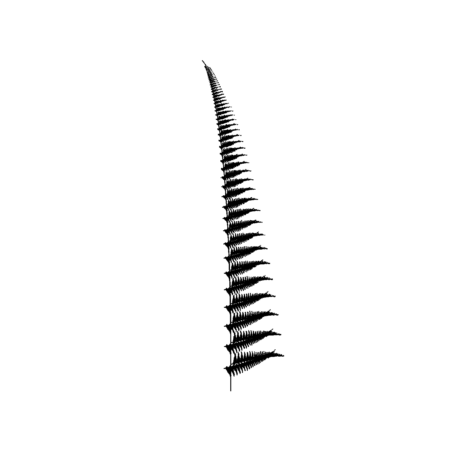
Tweetable barnsley fern
#rstats
m=matrix
z=0.2
K=list(m(c(0,0,0,z),2),m(c(0.8,-z,z,0.8),2),m(c(z,z,-z,z),2),m(c(-z,z,z,z),2))
k=list(c(0,0),c(0,2),c(0,2),c(0,0.4))
N=1e5
s=sample(1:4,N,T,c(1,85,7,7)/100)
P=m(0,2,N+1)
for (i in 1:N)P[,i+1]=K[[s[i]]]%*%P[,i]+k[[s[i]]]
plot(t(P),as=1,pch='.',ax=F,an=F)