devout 


devout is a package that enables R graphics devices to be written in plain R.
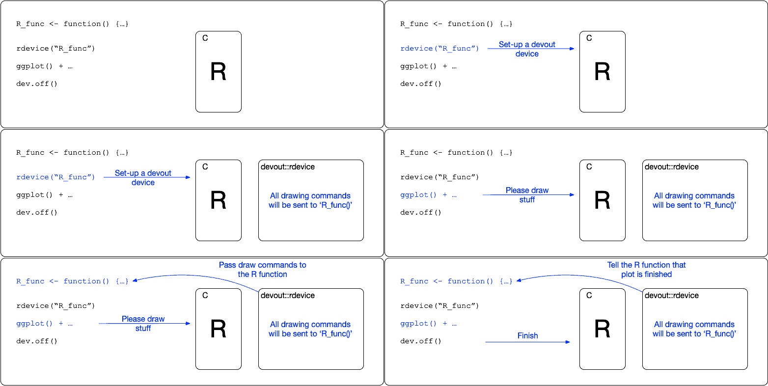
devout uses a pseudo-graphics-device which translates graphics
calls into a call to an R function of your design.
This means we can create alternative output devices (like pdf() or png()) using
only plain R.
How normal (C/C++) graphics devices work
animation (click to close)

How the devout device enables plain R graphics devices
animation (click to close)

What’s in the box
rdevice()- a generic device wrapper which will call the given R function to handle the graphics drawing.- Two example devices written in plain R (but using the underlying
rdevice())descriptive()- an output device which dumps information about the device calls.ascii()- a graphics device which outputs an ascii representation of the plot to a file, or to the console/terminal
How do I write my own graphics device?
If you want to write your own graphics device in plain R using devout you can:
- Read the
R/ascii-callback.Rincluded in the package - Read the vignettes.
A series of 4 vignettes are included in this package. They walk through the process of writing a naive SVG graphics device.
Installation
You can install from GitHub with:
# install.packages("remotes")
remotes::install_github("coolbutuseless/devout")
Simple device written in plain R: debug device
The following 5 lines of code are about the simplest device you can write with
devout in plain R.
This devices prints each of the device calls that were generated when the plot was “drawn”.
#~~~~~~~~~~~~~~~~~~~~~~~~~~~~~~~~~~~~~~~~~~~~~~~~~~~~~~~~~~~~~~~~~~~~~~~~~~~~~
# Write a function which takes 3 arguments
# @param device_call name of device function call
# @param args the arguments to that device call
# @param state current state of the graphics device
#~~~~~~~~~~~~~~~~~~~~~~~~~~~~~~~~~~~~~~~~~~~~~~~~~~~~~~~~~~~~~~~~~~~~~~~~~~~~~
debug_function <- function(device_call, args, state) {
  if (device_call %in% c('mode', 'strWidthUTF8', 'metricInfo')) return()
  cat("[", device_call, "]: ")
  cat(paste(names(args), args, sep = " = ", collapse = ",  "), "\n", sep = "")
}
#~~~~~~~~~~~~~~~~~~~~~~~~~~~~~~~~~~~~~~~~~~~~~~~~~~~~~~~~~~~~~~~~~~~~~~~~~~~~~
# Call the 'rdevice' and tell it that all calls should be passed to
# the above 'debug_function'
#~~~~~~~~~~~~~~~~~~~~~~~~~~~~~~~~~~~~~~~~~~~~~~~~~~~~~~~~~~~~~~~~~~~~~~~~~~~~~
rdevice('debug_function')
plot(1:10)
invisible(dev.off())[ open ]:
[ activate ]:
[ holdflush ]: level = 1
[ newPage ]:
[ clip ]: x0 = 59.04, y0 = 21526.56, x1 = 28769.76, y1 = 59.0400000000009
[ circle ]: x = 1122.4, y = 20731.4666666667, r = 2.7
[ circle ]: x = 4076.17777777778, y = 18522.8740740741, r = 2.7
[ circle ]: x = 7029.95555555556, y = 16314.2814814815, r = 2.7
[ circle ]: x = 9983.73333333334, y = 14105.6888888889, r = 2.7
[ circle ]: x = 12937.5111111111, y = 11897.0962962963, r = 2.7
[ circle ]: x = 15891.2888888889, y = 9688.5037037037, r = 2.7
[ circle ]: x = 18845.0666666667, y = 7479.91111111111, r = 2.7
[ circle ]: x = 21798.8444444444, y = 5271.31851851852, r = 2.7
[ circle ]: x = 24752.6222222222, y = 3062.72592592592, r = 2.7
[ circle ]: x = 27706.4, y = 854.133333333331, r = 2.7
[ clip ]: x0 = 0, y0 = 21600, x1 = 28800, y1 = 0
[ line ]: x1 = 4076.17777777778, y1 = 21526.56, x2 = 27706.4, y2 = 21526.56
[ line ]: x1 = 4076.17777777778, y1 = 21526.56, x2 = 4076.17777777778, y2 = 21533.76
[ line ]: x1 = 9983.73333333334, y1 = 21526.56, x2 = 9983.73333333334, y2 = 21533.76
[ line ]: x1 = 15891.2888888889, y1 = 21526.56, x2 = 15891.2888888889, y2 = 21533.76
[ line ]: x1 = 21798.8444444444, y1 = 21526.56, x2 = 21798.8444444444, y2 = 21533.76
[ line ]: x1 = 27706.4, y1 = 21526.56, x2 = 27706.4, y2 = 21533.76
[ textUTF8 ]: x = 4058.17777777778, y = 21552.48, str = 2, rot = 0, hadj = 0
[ textUTF8 ]: x = 9965.73333333334, y = 21552.48, str = 4, rot = 0, hadj = 0
[ textUTF8 ]: x = 15873.2888888889, y = 21552.48, str = 6, rot = 0, hadj = 0
[ textUTF8 ]: x = 21780.8444444444, y = 21552.48, str = 8, rot = 0, hadj = 0
[ textUTF8 ]: x = 27682.4, y = 21552.48, str = 10, rot = 0, hadj = 0
[ line ]: x1 = 59.04, y1 = 18522.8740740741, x2 = 59.04, y2 = 854.133333333331
[ line ]: x1 = 59.04, y1 = 18522.8740740741, x2 = 51.84, y2 = 18522.8740740741
[ line ]: x1 = 59.04, y1 = 14105.6888888889, x2 = 51.84, y2 = 14105.6888888889
[ line ]: x1 = 59.04, y1 = 9688.5037037037, x2 = 51.84, y2 = 9688.5037037037
[ line ]: x1 = 59.04, y1 = 5271.31851851852, x2 = 51.84, y2 = 5271.31851851852
[ line ]: x1 = 59.04, y1 = 854.133333333331, x2 = 51.84, y2 = 854.133333333331
[ textUTF8 ]: x = 41.76, y = 18540.8740740741, str = 2, rot = 90, hadj = 0
[ textUTF8 ]: x = 41.76, y = 14123.6888888889, str = 4, rot = 90, hadj = 0
[ textUTF8 ]: x = 41.76, y = 9706.5037037037, str = 6, rot = 90, hadj = 0
[ textUTF8 ]: x = 41.76, y = 5289.31851851852, str = 8, rot = 90, hadj = 0
[ textUTF8 ]: x = 41.76, y = 878.133333333331, str = 10, rot = 90, hadj = 0
[ polyline ]: n = 5, x = c(59.04, 28769.76, 28769.76, 59.04, 59.04), y = c(21526.56, 21526.56, 59.0400000000009, 59.0400000000009, 21526.56)
[ clip ]: x0 = 0, y0 = 21600, x1 = 28800, y1 = 0
[ textUTF8 ]: x = 14372.4, y = 21581.28, str = Index, rot = 0, hadj = 0
[ textUTF8 ]: x = 12.96, y = 10828.8, str = 1:10, rot = 90, hadj = 0
[ holdflush ]: level = -1
[ close ]: ascii() device
This is an example of a more complete graphics device. It is written in plain R and
relies on devout for all the interfacing with C++ and the internals of R.
The ascii() device draws an approximation of the graphics using ASCII characters
on the console (by default) or saved to a text file (if specified).
Limitations
- No support for: filled polygons, plotmath, alpha blending, angled text, rasters
- You should probably always add
theme(legend.position = 'none')because legends look awful in ascii.
ggplot2: Basic scatterplot
p <- ggplot(mtcars) +
  geom_point(aes(mpg, wt)) +
  labs(
    y     = "Car Weight",
    title    = "Basic scatter plot",
    subtitle = "Rendered with devout::ascii()"
  )  +
  theme_bw()

ascii(width = 100)
p
invisible(dev.off())
    Basic scatter plot
    Rendered with devout::ascii()
    +----------------------------------------------------------------------------------------------+
    |  .#       .       #.        .        .         .        .        .        .        .         |
    O..............................................................................................|
  5 |  .        .        .        .        .         .        .        .        .        .         |
    |  .        .        .        .        .         .        .        .        .        .         |
    |..............................................................................................|
    |  .        .        .        .        .         .        .        .        .        .         |
C 4 O.........................#....................................................................|
a   |  .        .  #     .#       #      # .         .        .        .        .        .         |
r   |..................#.#.#.......................................................................|
    |  .        .        .#       .##  # # .         .        .        .        .        .         |
W   |  .        .        .  #     .        .     #   .#     # .        .        .        .         |
e 3 O..........................................#...................................................|
i   |  .        .        .        .       #.   # #   .        .        .        .        .         |
g   |............................................#.................................................|
h   |  .        .        .        .        .         .#       .        .        .        #         |
t   O.............................................................#................................|
  2 |  .        .        .        .        .         .        .       #.        .        .     #   |
    |  .        .        .        .        .         .        .        .        . #      .         |
    |.............................................................................#................|
    +10O----------------15----------------20----------------25O----------------30----------------35O
                                                 mpg
pie plot in base R
ascii(width = 100)
pie(c(cool = 4, but = 2, use = 1, less = 8))
invisible(dev.off())


                                   but     ##############
                                       ####    #         ####  cool
                                    ###        #             ###
                                  ##            #               ##
                          use    ## ###         #                ##
                               ##      ###      #                  #
                               #          ###    #                  #
                               #########     ### #                  #
                              #         ##############################
                              #                                     #
                               #                                    #
                               ##                                  ##
                                ##                                ##
                                 ##                              ##
                                  ###                          ###
                                    ####                    ####
                                       #####            #####
                                            #############
                                          less
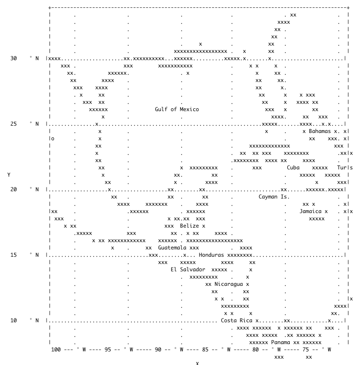
geom_sf() map of the Gulf of Mexico
geom_sf() example (click to open)
- Example taken from the r-spatial website
- This would probably look better with filled polygons, but they are not supported yet.
library(ggplot2)
library(sf)
library(rnaturalearth)
world <- ne_countries(scale = "medium", returnclass = "sf")

world_points <- st_centroid(world)
world_points <- cbind(world, st_coordinates(st_centroid(world$geometry)))

ascii(width = 200)
ggplot(data = world) +
  geom_sf() +
  geom_text(data= world_points,aes(x=X, y=Y, label=name),
            color = "darkblue", fontface = "bold", check_overlap = FALSE) +
  annotate(geom = "text", x = -90, y = 26, label = "Gulf of Mexico", fontface = "italic", color = "grey22", size = 6) +
  coord_sf(xlim = c(-102.15, -74.12), ylim = c(7.65, 33.97), expand = FALSE) +
  theme_bw()
invisible(dev.off())
Ideas for other Output Devices
- Colour ASCII/ANSI output
- Audio output
- HPGL plotting output
- CNC machine tooling instructions
- Directly drive motors to power an etch-a-sketch
News:
- v0.2.0 - Major refactor.
devoutis now a way of writing graphics devices in plain R with theascii()device as an example. - v0.1.2 - Added support for multiple page output
- v0.1.1 - Added support for path objects, so more map plots now work.
- v0.1.0 - initial release