ggplot2 geoms with support for pattern fills
Source:R/geom-rect.R, R/geom-bar.R, R/geom-bin2d.R, and 10 more
geom-docs.RdAll geoms in this package are identical to their counterparts in ggplot2 except that they can be filled with patterns.
geom_rect_pattern(
  mapping = NULL,
  data = NULL,
  stat = "identity",
  position = "identity",
  ...,
  linejoin = "mitre",
  na.rm = FALSE,
  show.legend = NA,
  inherit.aes = TRUE
)

geom_bar_pattern(
  mapping = NULL,
  data = NULL,
  stat = "count",
  position = "stack",
  ...,
  width = NULL,
  binwidth = NULL,
  na.rm = FALSE,
  orientation = NA,
  show.legend = NA,
  inherit.aes = TRUE
)

geom_histogram_pattern(
  mapping = NULL,
  data = NULL,
  stat = "bin",
  position = "stack",
  ...,
  binwidth = NULL,
  bins = NULL,
  na.rm = FALSE,
  orientation = NA,
  show.legend = NA,
  inherit.aes = TRUE
)

geom_bin2d_pattern(
  mapping = NULL,
  data = NULL,
  stat = "bin2d",
  position = "identity",
  ...,
  na.rm = FALSE,
  show.legend = NA,
  inherit.aes = TRUE
)

geom_boxplot_pattern(
  mapping = NULL,
  data = NULL,
  stat = "boxplot",
  position = "dodge2",
  ...,
  outlier.colour = NULL,
  outlier.color = NULL,
  outlier.fill = NULL,
  outlier.shape = 19,
  outlier.size = 1.5,
  outlier.stroke = 0.5,
  outlier.alpha = NULL,
  notch = FALSE,
  notchwidth = 0.5,
  varwidth = FALSE,
  na.rm = FALSE,
  orientation = NA,
  show.legend = NA,
  inherit.aes = TRUE
)

geom_col_pattern(
  mapping = NULL,
  data = NULL,
  position = "stack",
  ...,
  width = NULL,
  na.rm = FALSE,
  show.legend = NA,
  inherit.aes = TRUE
)

geom_crossbar_pattern(
  mapping = NULL,
  data = NULL,
  stat = "identity",
  position = "identity",
  ...,
  fatten = 2.5,
  na.rm = FALSE,
  orientation = NA,
  show.legend = NA,
  inherit.aes = TRUE
)

geom_ribbon_pattern(
  mapping = NULL,
  data = NULL,
  stat = "identity",
  position = "identity",
  ...,
  na.rm = FALSE,
  orientation = NA,
  show.legend = NA,
  inherit.aes = TRUE,
  outline.type = "both"
)

geom_area_pattern(
  mapping = NULL,
  data = NULL,
  stat = "identity",
  position = "stack",
  na.rm = FALSE,
  orientation = NA,
  show.legend = NA,
  inherit.aes = TRUE,
  ...,
  outline.type = "upper"
)

geom_density_pattern(
  mapping = NULL,
  data = NULL,
  stat = "density",
  position = "identity",
  ...,
  na.rm = FALSE,
  orientation = NA,
  show.legend = NA,
  inherit.aes = TRUE
)

geom_polygon_pattern(
  mapping = NULL,
  data = NULL,
  stat = "identity",
  position = "identity",
  rule = "evenodd",
  ...,
  na.rm = FALSE,
  show.legend = NA,
  inherit.aes = TRUE
)

geom_map_pattern(
  mapping = NULL,
  data = NULL,
  stat = "identity",
  ...,
  map,
  na.rm = FALSE,
  show.legend = NA,
  inherit.aes = TRUE
)

geom_sf_pattern(
  mapping = aes(),
  data = NULL,
  stat = "sf",
  position = "identity",
  na.rm = FALSE,
  show.legend = NA,
  inherit.aes = TRUE,
  ...
)

geom_tile_pattern(
  mapping = NULL,
  data = NULL,
  stat = "identity",
  position = "identity",
  ...,
  linejoin = "mitre",
  na.rm = FALSE,
  show.legend = NA,
  inherit.aes = TRUE
)

geom_violin_pattern(
  mapping = NULL,
  data = NULL,
  stat = "ydensity",
  position = "dodge",
  ...,
  draw_quantiles = NULL,
  trim = TRUE,
  scale = "area",
  na.rm = FALSE,
  orientation = NA,
  show.legend = NA,
  inherit.aes = TRUE
)
Arguments
- mapping
Set of aesthetic mappings created by
aes()oraes_(). If specified andinherit.aes = TRUE(the default), it is combined with the default mapping at the top level of the plot. You must supplymappingif there is no plot mapping.- data
The data to be displayed in this layer. There are three options:
If
NULL, the default, the data is inherited from the plot data as specified in the call toggplot().A
data.frame, or other object, will override the plot data. All objects will be fortified to produce a data frame. Seefortify()for which variables will be created.A
functionwill be called with a single argument, the plot data. The return value must be adata.frame, and will be used as the layer data. Afunctioncan be created from aformula(e.g.~ head(.x, 10)).- stat
Override the default connection between
geom_bar()andstat_count().- position
Position adjustment, either as a string, or the result of a call to a position adjustment function.
- ...
Other arguments passed on to
layer(). These are often aesthetics, used to set an aesthetic to a fixed value, likecolour = "red"orsize = 3. They may also be parameters to the paired geom/stat.- linejoin
Line join style (round, mitre, bevel).
- na.rm
If
FALSE, the default, missing values are removed with a warning. IfTRUE, missing values are silently removed.- show.legend
logical. Should this layer be included in the legends?
NA, the default, includes if any aesthetics are mapped.FALSEnever includes, andTRUEalways includes. It can also be a named logical vector to finely select the aesthetics to display.- inherit.aes
If
FALSE, overrides the default aesthetics, rather than combining with them. This is most useful for helper functions that define both data and aesthetics and shouldn't inherit behaviour from the default plot specification, e.g.borders().- width
Bar width. By default, set to 90% of the resolution of the data.
- binwidth
The width of the bins. Can be specified as a numeric value or as a function that calculates width from unscaled x. Here, "unscaled x" refers to the original x values in the data, before application of any scale transformation. When specifying a function along with a grouping structure, the function will be called once per group. The default is to use the number of bins in
bins, covering the range of the data. You should always override this value, exploring multiple widths to find the best to illustrate the stories in your data.The bin width of a date variable is the number of days in each time; the bin width of a time variable is the number of seconds.
- orientation
The orientation of the layer. The default (
NA) automatically determines the orientation from the aesthetic mapping. In the rare event that this fails it can be given explicitly by settingorientationto either"x"or"y". See the Orientation section for more detail.- bins
Number of bins. Overridden by
binwidth. Defaults to 30.- outlier.colour
Default aesthetics for outliers. Set to
NULLto inherit from the aesthetics used for the box.In the unlikely event you specify both US and UK spellings of colour, the US spelling will take precedence.
Sometimes it can be useful to hide the outliers, for example when overlaying the raw data points on top of the boxplot. Hiding the outliers can be achieved by setting
outlier.shape = NA. Importantly, this does not remove the outliers, it only hides them, so the range calculated for the y-axis will be the same with outliers shown and outliers hidden.- outlier.color
Default aesthetics for outliers. Set to
NULLto inherit from the aesthetics used for the box.In the unlikely event you specify both US and UK spellings of colour, the US spelling will take precedence.
Sometimes it can be useful to hide the outliers, for example when overlaying the raw data points on top of the boxplot. Hiding the outliers can be achieved by setting
outlier.shape = NA. Importantly, this does not remove the outliers, it only hides them, so the range calculated for the y-axis will be the same with outliers shown and outliers hidden.- outlier.fill
Default aesthetics for outliers. Set to
NULLto inherit from the aesthetics used for the box.In the unlikely event you specify both US and UK spellings of colour, the US spelling will take precedence.
Sometimes it can be useful to hide the outliers, for example when overlaying the raw data points on top of the boxplot. Hiding the outliers can be achieved by setting
outlier.shape = NA. Importantly, this does not remove the outliers, it only hides them, so the range calculated for the y-axis will be the same with outliers shown and outliers hidden.- outlier.shape
Default aesthetics for outliers. Set to
NULLto inherit from the aesthetics used for the box.In the unlikely event you specify both US and UK spellings of colour, the US spelling will take precedence.
Sometimes it can be useful to hide the outliers, for example when overlaying the raw data points on top of the boxplot. Hiding the outliers can be achieved by setting
outlier.shape = NA. Importantly, this does not remove the outliers, it only hides them, so the range calculated for the y-axis will be the same with outliers shown and outliers hidden.- outlier.size
Default aesthetics for outliers. Set to
NULLto inherit from the aesthetics used for the box.In the unlikely event you specify both US and UK spellings of colour, the US spelling will take precedence.
Sometimes it can be useful to hide the outliers, for example when overlaying the raw data points on top of the boxplot. Hiding the outliers can be achieved by setting
outlier.shape = NA. Importantly, this does not remove the outliers, it only hides them, so the range calculated for the y-axis will be the same with outliers shown and outliers hidden.- outlier.stroke
Default aesthetics for outliers. Set to
NULLto inherit from the aesthetics used for the box.In the unlikely event you specify both US and UK spellings of colour, the US spelling will take precedence.
Sometimes it can be useful to hide the outliers, for example when overlaying the raw data points on top of the boxplot. Hiding the outliers can be achieved by setting
outlier.shape = NA. Importantly, this does not remove the outliers, it only hides them, so the range calculated for the y-axis will be the same with outliers shown and outliers hidden.- outlier.alpha
Default aesthetics for outliers. Set to
NULLto inherit from the aesthetics used for the box.In the unlikely event you specify both US and UK spellings of colour, the US spelling will take precedence.
Sometimes it can be useful to hide the outliers, for example when overlaying the raw data points on top of the boxplot. Hiding the outliers can be achieved by setting
outlier.shape = NA. Importantly, this does not remove the outliers, it only hides them, so the range calculated for the y-axis will be the same with outliers shown and outliers hidden.- notch
If
FALSE(default) make a standard box plot. IfTRUE, make a notched box plot. Notches are used to compare groups; if the notches of two boxes do not overlap, this suggests that the medians are significantly different.- notchwidth
For a notched box plot, width of the notch relative to the body (defaults to
notchwidth = 0.5).- varwidth
If
FALSE(default) make a standard box plot. IfTRUE, boxes are drawn with widths proportional to the square-roots of the number of observations in the groups (possibly weighted, using theweightaesthetic).- fatten
A multiplicative factor used to increase the size of the middle bar in
geom_crossbar()and the middle point ingeom_pointrange().- outline.type
Type of the outline of the area;
"both"draws both the upper and lower lines,"upper"/"lower"draws the respective lines only."full"draws a closed polygon around the area.- rule
Either
"evenodd"or"winding". If polygons with holes are being drawn (using thesubgroupaesthetic) this argument defines how the hole coordinates are interpreted. See the examples ingrid::pathGrob()for an explanation.- map
Data frame that contains the map coordinates. This will typically be created using
fortify()on a spatial object. It must contain columnsxorlong,yorlat, andregionorid.- draw_quantiles
If
not(NULL)(default), draw horizontal lines at the given quantiles of the density estimate.- trim
If
TRUE(default), trim the tails of the violins to the range of the data. IfFALSE, don't trim the tails.- scale
if "area" (default), all violins have the same area (before trimming the tails). If "count", areas are scaled proportionally to the number of observations. If "width", all violins have the same maximum width.
Value
A ggplot2::Geom object.
Pattern Arguments
Not all arguments apply to all patterns.
patternPattern name string e.g. 'stripe' (default), 'crosshatch', 'point', 'circle', 'none'
pattern_alphaAlpha transparency for pattern. default: 1
pattern_angleOrientation of the pattern in degrees. default: 30
pattern_aspect_ratioAspect ratio adjustment.
pattern_colourColour used for strokes and points. default: 'black'
pattern_densityApproximate fill fraction of the pattern. Usually in range [0, 1], but can be higher. default: 0.2
pattern_filenameImage filename/URL.
pattern_fillFill colour. default: 'grey80'
pattern_fill2Second fill colour. default: '#4169E1'
pattern_filter(Image scaling) filter. default: 'lanczos'
pattern_frequencyFrequency. default: 0.1
pattern_gravityImage placement. default: 'center'
pattern_gridPattern grid type. default: 'square'
pattern_key_scale_factorScale factor for pattern in legend. default: 1
pattern_linetypeStroke linetype. default: 1
pattern_option_1Generic user value for custom patterns.
pattern_option_2Generic user value for custom patterns.
pattern_option_3Generic user value for custom patterns.
pattern_option_4Generic user value for custom patterns.
pattern_option_5Generic user value for custom patterns.
pattern_orientation'vertical', 'horizontal', or 'radial'. default: 'vertical'
pattern_resPattern resolution (pixels per inch).
pattern_rotRotation angle (shape within pattern). default: 0
pattern_scaleScale. default: 1
pattern_shapePlotting shape. default: 1
pattern_sizeStroke line width. default: 1
pattern_spacingSpacing of the pattern as a fraction of the plot size. default: 0.05
pattern_typeGeneric control option
pattern_subtypeGeneric control option
pattern_xoffsetOffset the origin of the pattern. Range [0, 1]. default: 0. Use this to slightly shift the origin of the pattern. For most patterns, the user should limit the offset value to be less than the pattern spacing.
pattern_yoffsetOffset the origin of the pattern. Range [0, 1]. default: 0. Use this to slightly shift the origin of the pattern. For most patterns, the user should limit the offset value to be less than the pattern spacing.
Examples
if (require("ggplot2")) {
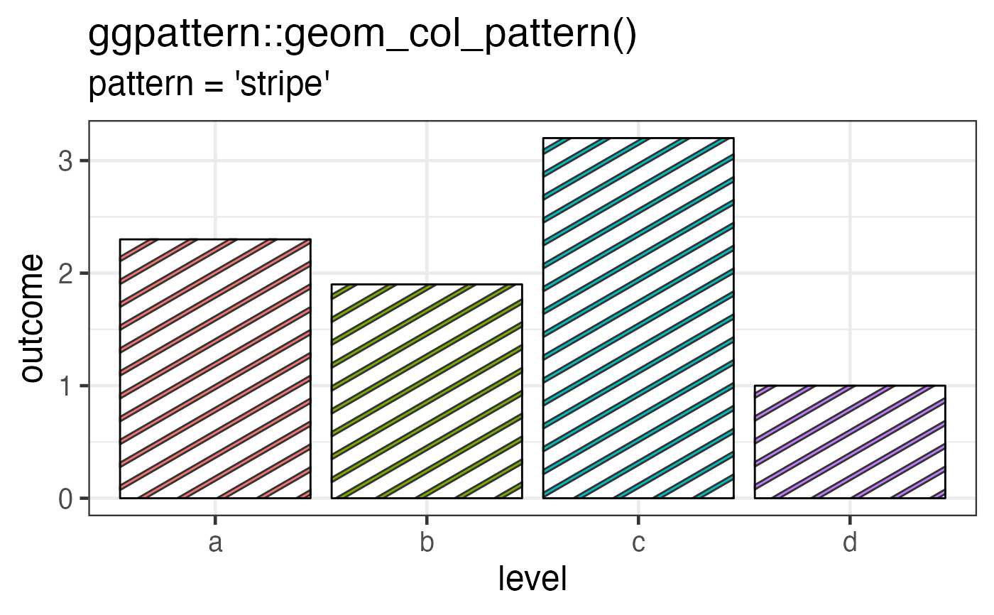
# 'stripe' pattern example
df <- data.frame(level = c("a", "b", "c", 'd'), outcome = c(2.3, 1.9, 3.2, 1))
gg <- ggplot(df) +
geom_col_pattern(
aes(level, outcome, pattern_fill = level),
pattern = 'stripe',
fill = 'white',
colour = 'black'
) +
theme_bw(18) +
theme(legend.position = 'none') +
labs(
title = "ggpattern::geom_col_pattern()",
subtitle = "pattern = 'stripe'"
)
plot(gg)
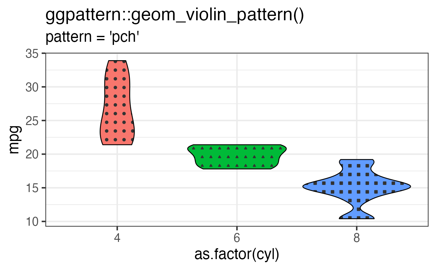
# 'pch' pattern example
gg <- ggplot(mtcars, aes(as.factor(cyl), mpg)) +
geom_violin_pattern(aes(fill = as.factor(cyl),
pattern_shape = as.factor(cyl)),
pattern = 'pch',
pattern_density = 0.3,
pattern_angle = 0,
colour = 'black'
) +
theme_bw(18) +
theme(legend.position = 'none') +
labs(
title = "ggpattern::geom_violin_pattern()",
subtitle = "pattern = 'pch'"
)
plot(gg)
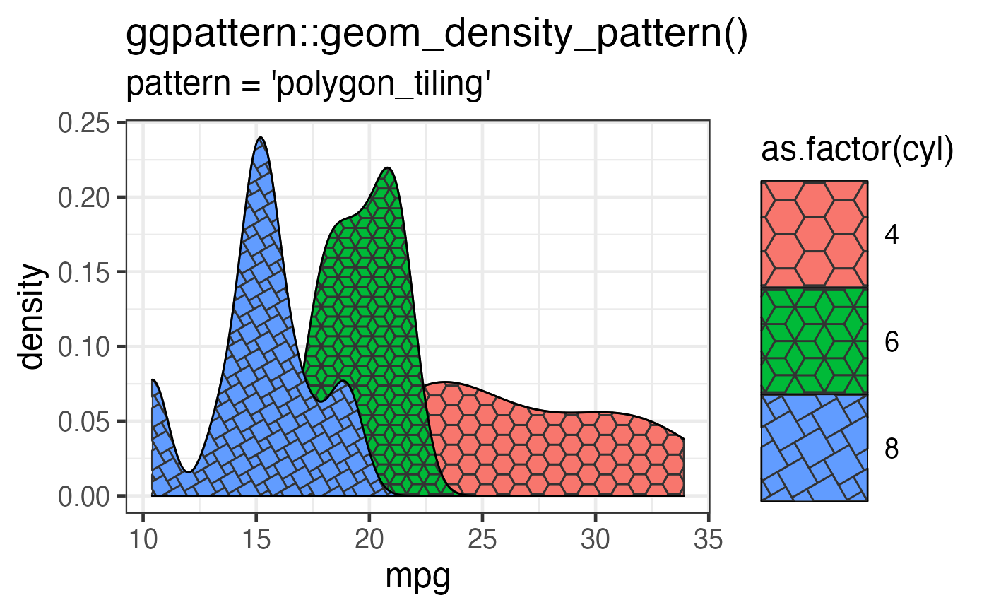
# 'polygon_tiling' pattern example
gg <- ggplot(mtcars) +
geom_density_pattern(
aes(
x = mpg,
pattern_fill = as.factor(cyl),
pattern_type = as.factor(cyl)
),
pattern = 'polygon_tiling',
pattern_key_scale_factor = 1.2
) +
scale_pattern_type_manual(values = c("hexagonal", "rhombille",
"pythagorean")) +
theme_bw(18) +
theme(legend.key.size = unit(2, 'cm')) +
labs(
title = "ggpattern::geom_density_pattern()",
subtitle = "pattern = 'polygon_tiling'"
)
plot(gg)
}