nara is a package for working with R’s native raster image format.
Native raster images are fast to manipulate and render, and open the possibility for realtime rendering e.g. games and interactive applications.
nara:
- uses C to speed up operations
- uses in-place operations to avoid memory allocations.
- renders discrete, non-aliased pixels (internally all coordinates are rounded to integer values)
- includes basic drawing primitives e.g. rectangles, lines, circles
What’s in the box
- Image creation
- Conversion
- Drawing
- Selection and Combination
- Color manipulation
- Sample images
deer
Reading and writing native raster images is supported by jpeg, png, and fastpng packages.
Installation
You can install from GitHub with:
# install.package('remotes')
remotes::install_github('coolbutuseless/nara')
Demonstration
Realtime rendering of a forest (made of 11 overlapping parallax layers with alpha blending) with a samurai figure running out front.
https://github.com/user-attachments/assets/c3daeccc-0d21-4f0d-ba1e-655fd836c9c3
Static Rendering: Example
The following is a rendering of a single scene with multiple elements.
The interesting thing about this scene that drawing all the objects into the native raster image and rendering to screen can take as little as 5 millseconds.
This means that this scene could render at around 200 frames-per-second.
library(grid)
library(nara)
set.seed(1)

#~~~~~~~~~~~~~~~~~~~~~~~~~~~~~~~~~~~~~~~~~~~~~~~~~~~~~~~~~~~~~~~~~~~~~~~~~~~~~
# Create 'nr' image
#~~~~~~~~~~~~~~~~~~~~~~~~~~~~~~~~~~~~~~~~~~~~~~~~~~~~~~~~~~~~~~~~~~~~~~~~~~~~~
w  <- 10
h  <- 8
nr <- nr_new(w * 30, h * 30, fill = 'grey98')

#~~~~~~~~~~~~~~~~~~~~~~~~~~~~~~~~~~~~~~~~~~~~~~~~~~~~~~~~~~~~~~~~~~~~~~~~~~~~~
# Draw a grid of squares
#~~~~~~~~~~~~~~~~~~~~~~~~~~~~~~~~~~~~~~~~~~~~~~~~~~~~~~~~~~~~~~~~~~~~~~~~~~~~~
colors <- viridisLite::inferno(w * h)
coords  <- expand.grid(y = seq(0, h-1) * 30 + 1, x = seq(0, w-1) * 30 + 1)
nr_rect(nr, x = coords$x, y = coords$y, w = 27, h = 27, fill = colors)

#~~~~~~~~~~~~~~~~~~~~~~~~~~~~~~~~~~~~~~~~~~~~~~~~~~~~~~~~~~~~~~~~~~~~~~~~~~~~~
# Draw a bunch of deer sprites
#~~~~~~~~~~~~~~~~~~~~~~~~~~~~~~~~~~~~~~~~~~~~~~~~~~~~~~~~~~~~~~~~~~~~~~~~~~~~~
nr_blit(dst = nr, src = deer[[1]],
        x = sample(300, 15), y = sample(200, 15))


#~~~~~~~~~~~~~~~~~~~~~~~~~~~~~~~~~~~~~~~~~~~~~~~~~~~~~~~~~~~~~~~~~~~~~~~~~~~~~
# Add an image read from file (with alpha transparency)
#~~~~~~~~~~~~~~~~~~~~~~~~~~~~~~~~~~~~~~~~~~~~~~~~~~~~~~~~~~~~~~~~~~~~~~~~~~~~~
img <- fastpng::read_png(system.file("image/deer-1.png", package = "nara"), type = 'nativeraster')
img <- nr_scale(img, 0.15)
nr_blit(dst = nr, src = img, x = 50, y = 50)

#~~~~~~~~~~~~~~~~~~~~~~~~~~~~~~~~~~~~~~~~~~~~~~~~~~~~~~~~~~~~~~~~~~~~~~~~~~~~~
# Add a polygon
#~~~~~~~~~~~~~~~~~~~~~~~~~~~~~~~~~~~~~~~~~~~~~~~~~~~~~~~~~~~~~~~~~~~~~~~~~~~~~
thetas <- seq(pi/6, 2*pi, pi/3)
x <- 50 * cos(thetas) + 240
y <- 50 * sin(thetas) + 180
nr_polygon(nr, x = x, y = y, fill = '#556688c0', color = 'blue')

#~~~~~~~~~~~~~~~~~~~~~~~~~~~~~~~~~~~~~~~~~~~~~~~~~~~~~~~~~~~~~~~~~~~~~~~~~~~~~
# Add text to the image
#~~~~~~~~~~~~~~~~~~~~~~~~~~~~~~~~~~~~~~~~~~~~~~~~~~~~~~~~~~~~~~~~~~~~~~~~~~~~~
nr_text_basic(nr, x = 180, y = 20, str = "Hello #RStats", fontsize = 16)

#~~~~~~~~~~~~~~~~~~~~~~~~~~~~~~~~~~~~~~~~~~~~~~~~~~~~~~~~~~~~~~~~~~~~~~~~~~~~~
# Copy image to the device
#~~~~~~~~~~~~~~~~~~~~~~~~~~~~~~~~~~~~~~~~~~~~~~~~~~~~~~~~~~~~~~~~~~~~~~~~~~~~~
plot(nr)
Static Rendering: Displaying Sprites
Included with nara are 16 frames of an animated deer character - see deer data.
Blit the first deer frame onto a native raster canvas.
nr <- nr_new(100, 32, 'grey80')
nr_blit(dst = nr, src = deer[[1]], x = 2, y = 0, hjust = 0, vjust = 0)
plot(nr)
Dynamic (realtime) Rendering: Animated deer
The reason to use nara is that operations are fast enough that native raster images can be used as an in-memory buffer for a double-bufferred rendering system.
Double-buffered rendering is where two buffers are used for rendering with one buffer being shown to the user, and the other existing in memory as a place to render.
In this example, the deer sprite is rendered to a larger native raster image. This in-memory buffer is then displayed to the user using plot() (which just wraps a call to grid.raster()).
By altering the position and animation frame every time the kind is shown, smooth animation is possible.
This simple code runs at well over 100 frames-per-second.
It is unlikely your screen will refresh this fast, but it does indicate that there is plenty of headroom for more complicated computations for each frame.
library(grid)

# Setup a fast graphics device that can render quickly
x11(type = 'cairo', antialias = 'none')
dev.control('inhibit')

# Create the in-memory native raster image
nr <- nr_new(100, 32, 'grey80')

# Clear, blit and render => animation!
for (i in -30:110) {
  nr_fill(nr, 'grey80')                    # Clear the native raster image
  sprite_idx <- floor((i/3) %% 5) + 11
  nr_blit(dst = nr, src = deer[[sprite_idx]], x = i, y = 15) # copy deer to the image
  plot(nr)
  Sys.sleep(0.03)                          # Stop animation running too fast.
}
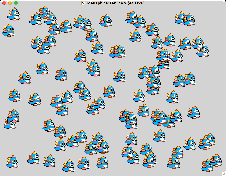
Working with multiple sprites
You can quickly blit (i.e. copy) a sprite into multiple locations on the nativeraster with nr_blit() and nr_blit_list()
In this example 100 random positions and velocities are first created. A character sprite is then blitted to each of these 100 locations.
The positions are updated using the velocities, and the next frame is rendered. In this way multiple sprites are rendered and animated on screen.
library(grid)

# Setup a fast graphics device that can render quickly
x11(type = 'dbcairo', antialias = 'none', width = 8, height = 6)
dev.control('inhibit')

# Number of sprites
N <- 100

# Canvas size
w <- 400
h <- 300

# location and movement vector of all the sprites
x  <- sample(w, N, replace = TRUE)
y  <- sample(h, N, replace = TRUE)
vx <- runif(N, 1, 5)


# Create an empty nativeraster with a grey background
nr <- nr_new(w, h, 'white')


for (frame in 1:1000) {
  # Clear the nativeraster and blit in all the deer
  nr_fill(nr, 'white')
  deer_idx <- floor((frame/3) %% 5 + 11)
  nr_blit(dst = nr, src = deer[[deer_idx]], x, y)

  # Draw the nativeraster to screen
  plot(nr)

  # Update the position of each deer.
  # Position wraps around
  x <- x + vx
  x <- ifelse(x > w , -32, x)

  # slight pause. Otherwise everything runs too fast!
  Sys.sleep(0.03)
}
Technical bits
What is a native raster image and why is it fast?
A native raster image is a built-in datatype in R.
It is an integer matrix where each integer represents the RGBA color at a single pixel. The 32-bit integer at each location is interpreted within R to be four color channels (RGBA) represented by 8 bits each.
This way of encoding color information is closer to the internal representation used by graphics devices, and therefore can be faster to render and manipulate.
Native rasters do not use pre-multiplied alpha.
In-place operation
nara is targeted at fast rendering (>30fps), and tries to minimise R function calls and memory allocations.
When updating native raster image with this package, changes are done in place on the current image i.e. a new image is not created.
Anti-aliasing/Interpolation
No anti-aliasing is done by the draw methods in this package.
No interpolation is done - x and y values for drawing coordinates are always rounded to integers.
Dimension ordering
All arguments specifying dimensions are in the order horizontal then vertical i.e.
- x, y
- width, height
- hjust, vjust
Coordinate System
The coordinate system for nara native raster image has the origin at the top left corner with coordinates (0, 0).
This is equivalent to {grid} graphics using native units.
It is also how magick represents image coordinates, as well as the majority of C graphics libraries.