svg-with-d3

library(devoutsvg)
#> Loading required package: devout

Introduction

This example is an adapted version of timelyportfolio’s interactive version of a plot originally by Claus Wilke.

My input here is minimal. The D3 javascript code is taken almost verbatim from timelyportfolio’s examples:

• example 1
• example 2

The difference with this {devoutsvg} example is that the d3 code is injected into the plot during the process of rendering to device. While in timelyportfolio’s examples, the plot is output to SVG, the SVG is then read back in and manipulated as a character string, and then written back out.

Code

# will need newest ggplot2, github multiscales, and dev version of colorspace
# install.packages('ggplot2')
# install.packages("colorspace", repos = "http://R-Forge.R-project.org")
# devtools::install_github("clauswilke/multiscales")

# http://bl.ocks.org/timelyportfolio/47cac2df130436f3292afaa38253072d/9bde7a2417cc44b3b14038a6a945f604960cef87

library(htmltools)
library(ggplot2)
library(d3r)
library(multiscales)
#> Note: The package "multiscales" is highly experimental. Use at your own risk.
#> 
#> Attaching package: 'multiscales'
#> The following object is masked from 'package:utils':
#> 
#>     zip
library(class)
library(KernSmooth)
#> KernSmooth 2.23 loaded
#> Copyright M. P. Wand 1997-2009

# example from Claus Wilke's multiscales README
colors <- scales::colour_ramp(
  colors = c(red = "#AC202F", purple = "#740280", blue = "#2265A3")
)((0:7)/7)

ggp <- ggplot(US_polling) + 
  geom_sf(aes(fill = zip(Clinton_lead, moe_normalized)), color = "gray30", size = 0.2) + 
  coord_sf(datum = NA) +
  bivariate_scale("fill",
                  pal_vsup(values = colors, max_desat = 0.8, pow_desat = 0.2, max_light = 0.7, pow_light = 1),
                  name = c("Clinton lead", "uncertainty"),
                  limits = list(c(-40, 40), c(0, 1)),
                  breaks = list(c(-40, -20, 0, 20, 40), c(0, 0.25, 0.50, 0.75, 1.)),
                  labels = list(waiver(), scales::percent),
                  guide = "colourfan"
  ) +
  theme_void() +
  theme(
    legend.key.size = grid::unit(0.8, "cm"),
    legend.title.align = 0.5,
    plot.margin = margin(5.5, 20, 5.5, 5.5)
  )

ggp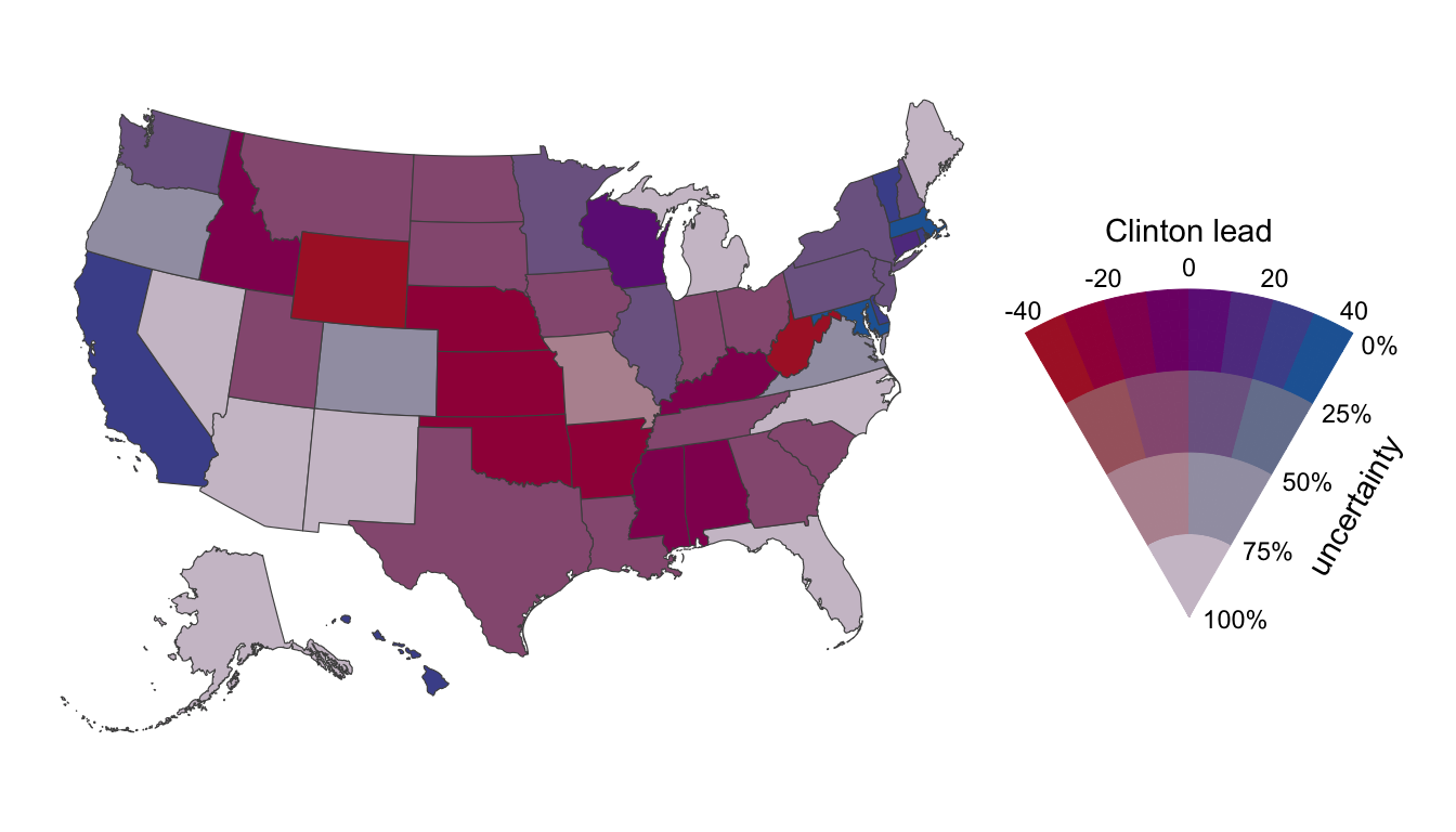

my_js_code <- "  
var svg = d3.select('svg')

  // add original fill as data on each state path
  svg.selectAll('path').each( function(d) {
    d3.select(this).datum({color: d3.select(this).style('fill')})
  })

  // this is not necessary but makes it cleaner
  //   add g group for each polygon in the legend
  //   the polygons are multiple small portions of the space in the legend
  //   rather than one polygon for each color
  var legendcolors = d3.set()
  svg.selectAll('polygon').each(function(d){legendcolors.add(d3.select(this).style('fill'))})

  legendcolors.values().forEach(function(color) {
    var g = svg.insert('g','svg>polygon').classed('legend-color',true).datum({color: color})
    svg.selectAll('polygon')
      .filter(function(d) {return d3.select(this).style('fill') === color})
      .each(function(d) {
        g.node().appendChild(this)
      })
  })

  svg.selectAll('g.legend-color').on('mouseover', function(d) {
    svg.selectAll('path').filter(pathd => pathd.color !== d.color).style('fill', 'white')
    svg.selectAll('path').filter(pathd => pathd.color === d.color).style('fill', d.color)
  })

  svg.selectAll('g.legend-color').on('mouseout', function(d) {
    svg.selectAll('path').style('fill', pathd => pathd.color)
  })
"

svgfile <- tempfile(fileext = ".svg")
devoutsvg::svgout(
  filename     = svgfile, 
  js_url       = "https://d3js.org/d3.v5.min.js",
  js_code      = my_js_code
)
ggp
invisible(dev.off())

htmltools::includeHTML(svgfile)