svg-with-gradient-fill

#~~~~~~~~~~~~~~~~~~~~~~~~~~~~~~~~~~~~~~~~~~~~~~~~~~~~~~~~~~~~~~~~~~~~~~~~~~~~
# install devout and its dependencies
#
# svgpatternsimple - a set of simple patterns in SVG
# devout           - Framework for creating graphics devices in plain R
# devoutsvg        - Custom SVG device
#~~~~~~~~~~~~~~~~~~~~~~~~~~~~~~~~~~~~~~~~~~~~~~~~~~~~~~~~~~~~~~~~~~~~~~~~~~~~
# devtools::install_github("coolbutuseless/svgpatternsimple") 
# devtools::install_github("coolbutuseless/devout")    
# devtools::install_github("coolbutuseless/devoutsvg") 

suppressPackageStartupMessages({
  library(devout)
  library(devoutsvg)
  library(svgpatternsimple)
  
  library(dplyr)
  library(tidyr)
  library(ggplot2)
  library(ggridges)
})

Deaths Of Drug Poisoning

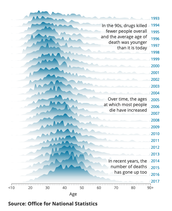
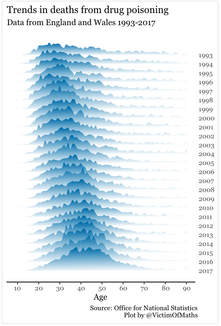
This vignette recreates a plot with vertical colour gradient. It was developed by VictimOfMaths and the complete version is available on github.

The image below on the left is from the UK Office for National Statistics (ONS).

The image on the right is created using R, ggplot and devoutsvg

Simple gradient example

Create, view, debug and iterate to find a gradient fill of your liking.

#~~~~~~~~~~~~~~~~~~~~~~~~~~~~~~~~~~~~~~~~~~~~~~~~~~~~~~~~~~~~~~~~~~~~~~~~~~~~
# Create SVG gradient pattern definition
#~~~~~~~~~~~~~~~~~~~~~~~~~~~~~~~~~~~~~~~~~~~~~~~~~~~~~~~~~~~~~~~~~~~~~~~~~~~~
gradient_pattern <- svgpatternsimple::create_pattern_gradient(
  id      = "p1",      # HTML/SVG id to assign to this pattern
  angle   = 90,        # Direction of the gradient
  colour1 = "White",   # Starting colour
  colour2 = "#0570b0"  # Final colour
)

# Contents of 'gradient_pattern'
#> <linearGradient id="p1" x1="0%" y1="100%" x2="0%" y2="0%">
#>   <stop style="stop-color:White;stop-opacity:1" offset="0%" />
#>   <stop style="stop-color:#0570b0;stop-opacity:1" offset="100%" />
#> </linearGradient>

# Visualise in viewer in Rstudio
# gradient_pattern$show()

my_pattern_list <- list(
  `#000001` = list(fill = gradient_pattern)
)


#~~~~~~~~~~~~~~~~~~~~~~~~~~~~~~~~~~~~~~~~~~~~~~~~~~~~~~~~~~~~~~~~~~~~~~~~~~~~
# Render the graph to the 'svgout' device and nominate any patterns to be 
# rendered by the 'svgpatternsimple' package
#~~~~~~~~~~~~~~~~~~~~~~~~~~~~~~~~~~~~~~~~~~~~~~~~~~~~~~~~~~~~~~~~~~~~~~~~~~~~
svgout(filename = "svg/test-gradient.svg", pattern_list = my_pattern_list)
  ggplot(iris, aes(x=Sepal.Width, y=Species)) +
  geom_density_ridges(alpha=0.33, scale=2, fill='#000001', colour=alpha(0.1)) +
  theme_classic()
#> Picking joint bandwidth of 0.13
invisible(dev.off())    

Recreate the ONS Plot

• Grab the raw data from the ONS
• Reshape into tidy form
• Create a ggridges plot
  • Use the devoutsvg device with svgpatternsimple
  • Use the encoded gradient created above (i.e. gradRGB) as the fill colour for the ridges.

#~~~~~~~~~~~~~~~~~~~~~~~~~~~~~~~~~~~~~~~~~~~~~~~~~~~~~~~~~~~~~~~~~~~~~~~~~~~~
# Read (and cache) the data from the ONS 
#~~~~~~~~~~~~~~~~~~~~~~~~~~~~~~~~~~~~~~~~~~~~~~~~~~~~~~~~~~~~~~~~~~~~~~~~~~~~
# drugs <- readr::read_csv("https://www.ons.gov.uk/visualisations/dvc661/drugs/datadownload.csv"   )
# saveRDS(drugs, "data/drugs.rds")
drugs <- readRDS("data/drugs.rds")

#~~~~~~~~~~~~~~~~~~~~~~~~~~~~~~~~~~~~~~~~~~~~~~~~~~~~~~~~~~~~~~~~~~~~~~~~~~~~
# Tidy + reshape data
#~~~~~~~~~~~~~~~~~~~~~~~~~~~~~~~~~~~~~~~~~~~~~~~~~~~~~~~~~~~~~~~~~~~~~~~~~~~~
drugs <- drugs %>%
  mutate(
    Age = case_when(
      Age   == "<10" ~ "9",
      Age   == "90+" ~ "90",
      TRUE  ~  Age
    )
  ) %>%
  tidyr::gather("Year", "Deaths", -Age) %>%
  mutate(
    Age  = as.integer(Age),
    Year = as.integer(Year)
  )


#~~~~~~~~~~~~~~~~~~~~~~~~~~~~~~~~~~~~~~~~~~~~~~~~~~~~~~~~~~~~~~~~~~~~~~~~~~~~
# Render the graph to the 'svgout' device and nominate any fill colours to be 
# rendered by the 'svgpatternsimple' package
#~~~~~~~~~~~~~~~~~~~~~~~~~~~~~~~~~~~~~~~~~~~~~~~~~~~~~~~~~~~~~~~~~~~~~~~~~~~~
svgout(filename = "svg/DrugDeaths.svg", pattern_list = my_pattern_list, width=4, height=6)
ggplot(drugs, aes(Age, Year, height=Deaths, group=Year)) +
  geom_density_ridges(stat='identity', scale = 3, colour=NA, fill='#000001') + 
  scale_y_reverse(position = 'right', breaks = sort(unique(drugs$Year))) +
  scale_x_continuous(breaks = seq(10, 90, 10)) +
  theme_classic() +
  theme(
    axis.line.y  = element_blank(), 
    axis.ticks.y = element_blank(), 
    axis.title.y = element_blank(),
    text         = element_text(family="Georgia")
  ) +
  labs(
    title    = "Trends in deaths from drug poisoning",
    subtitle = "Data from England and Wales 1993-2017",
    caption  = "Source: Office for National Statistics\nPlot by @VictimOfMaths"
  )
invisible(dev.off())